User Manual: GenerationOne MCS
1. Introduction
This manual is intended to be used as a reference on how to use the Bright Ascension Mission Control System (MCS). The MCS is a desktop application used for operating a spacecraft that uses Bright Ascension’s FSDK.
1.1. How this manual is structured
The MCS user manual is structured to be used as a reference whilst using the MCS. The manual starts with a brief overview of the core concepts and views within the MCS and then leads into the various core uses such as monitoring and housekeeping.
Section 4 and onwards describe general uses of the MCS in depth.
-
Section 4 (Monitoring) shows how you can examine telemetry received from the spacecraft in various forms and contexts.
-
Section 5 (Transfers) shows how transfers can be made to and from the satellite and how these transfers are monitored.
-
Section 6 (Scripting) describes the scripting interface within the MCS and describes how scripts are written for use inside the MCS. Scripts are integral for the chapter on scheduling.
-
Section 7 (External Scripting) describes the Python API which can be used to execute MCS functions via external Python scripts.
-
Section 8 (The Ground Schedule) and Section 9 (The On-Board Schedule) explain how the ground-side and flight-side schedules are administered inside the MCS.
-
Section 10 (Calibrations & Checks) explains how to set calibrations to convert from raw parameter values to calibrated parameter values and adding checks to highlight check exceptions for parameter values.
-
Section 11 (Configuration) lists the configuration settings which can be used to set MCS data locations and behaviour.
-
Section 12 (Housekeeping) explains how to monitor housekeeping packets and how to make sense of aggregated data.
-
Section 13 (Decoding data) explains the various tools within the MCS available to decode aggregations, data logs and events.
-
Section 14 (Archiving) explains what data is archived and how to access it.
-
Section 15 (Time Correlation) explains how to set the ground parameters which MCS uses to convert between On-Board Time values and UTC.
-
Section 16 (Ground Station Networks) describes how to set up the MCS to communicate via supported third-party Ground Station Networks - currently KSatLite and LeafSpace.
-
Section 17 (Export and Import) describes how MCS configuration settings can be exported and imported, for backup or sharing of settings between installations.
-
Section 18 (Synthetic Parameters) describes how to define and manage parameters whose values are derived from one or more other parameters.
-
Section 19 (Procedure execution) describes what procedure execution is and how to define, manage and execute procedures
1.2. How to use this manual
Depending on what you need and your current familiarity with the MCS you may want to selectively read some chapters.
For complete beginners it’s recommended to read the Section 2 (Overview) which will give you a foundational overview of the MCS. If you want to get out of the theory, Section 3 (Getting started) will guide you through to the stage of connecting and doing basic interaction with the spacecraft. Further sections can be read when knowledge of the particular topic is required.
1.3. Installation
The installation of MCS is a simple process of extracting archives and, optionally, performing some initial basic configuration.
1.3.1. System Requirements
The following software requirements must be met before installation of the MCS is possible:
| Java Runtime Environment (JRE) | Version 11 |
|---|---|
Operating System |
Ubuntu version 16.04 LTS or higher |
Microsoft Windows 10 |
1.3.2. Installation procedure
The MCS is a client-server application. Both the client (display) and the server are delivered as Zip files, each containing a distribution of the MCS software and associated configuration files. The MCS client must be installed and run in order to access any MCS functionality. The MCS client can be installed on the same system as the server, and/or on other systems with a network connection to the server’s system.
For both client and client, the first steps of installation are:
-
Ensure the Java JRE is installed and is part of your path.
-
Extract the distribution archive in any directory.
1.4. Running
Each distribution contains helper scripts (for Windows and Unix) for launching the application, as listed in Helper scripts for Ubuntu and Windows operating systems.. A licence file is needed with a valid licence code in order to run the MCS. This can be obtained by contacting BAL. The licence file (licence.properties) needs to be in a folder called 'licence' in your MCS Server installation area.
| Operating System: | Ubuntu | Windows |
|---|---|---|
MCS Server |
|
|
MCS Display |
|
|
Once the MCS client is running and initialised, multiple instances of the MCS Display can be run simultaneously, and connect to the server. On first starting each client (Display), a connection dialog is displayed, allowing you to enter the address and TCP port of the client (Figure 1).
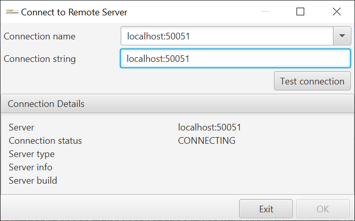
This allows you to enter multiple MCS client locations, and save them as named connections. Holding the Shift key on startup allows you to select which MCS client to connect to from the saved list, or add a new entry. After editing or selecting the connection details, press the Test connection button, and if an MCS client is found at the specified location, the server details will be displayed (Figure 2), and the OK button enabled, so you can press it to connect to the selected server.
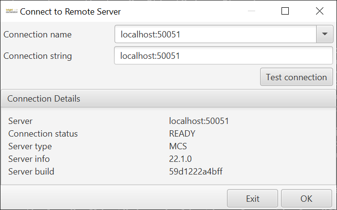
If you do not press the Shift key, the Display application will automatically connect to the last client it connected to.
1.4.1. Command line options
It is possible to provide system properties as command line arguments forming part of the run command which customise the behaviour of MCS. System properties should be provided prefixed with -D and can be added to the helper scripts. A list of the available system properties can be seen in A summary of the command-line options available when running the MCS..
| System property | Effect | Default |
|---|---|---|
|
(Display) Default location for file browser dialogs |
|
|
(Server) Archive file location |
|
2. Overview
The following chapter serves to provide you with an understanding of the fundamental components of the MCS user interface and how to use these components effectively to interact with your spacecraft.
The MCS provides a graphical user interface for communicating with the Gen1 on-board software (OBSW), it interacts with the OBSW through the various components provided by the OBSW. A component is made up of parameters and actions, and it is through these that we can interact with the spacecraft.
The various areas of the main user interface are described in the following sections.
2.1. Menu Bar
The menu bar at the top provides access to many functions described in this manual. The current time according to the MCS Server’s configured time zone (see Section 11.1.1) is displayed at the right of this area. Broadly, File contains core MCS and mission settings, Housekeeping deals with aggregations, beacons and archiving, Monitor covers activities and parameters both historical and current, Tools has schedule builders, log decoders, and synthetic parameters, and Help a brief aid in running the MCS.
| The various options and functionality in the menu will be highlighted as the relevant topic is covered in detail in further chapters. |
2.2. Toolbar
The toolbar, below the menu bar as highlighted in Figure 3, provides access to core functionality.
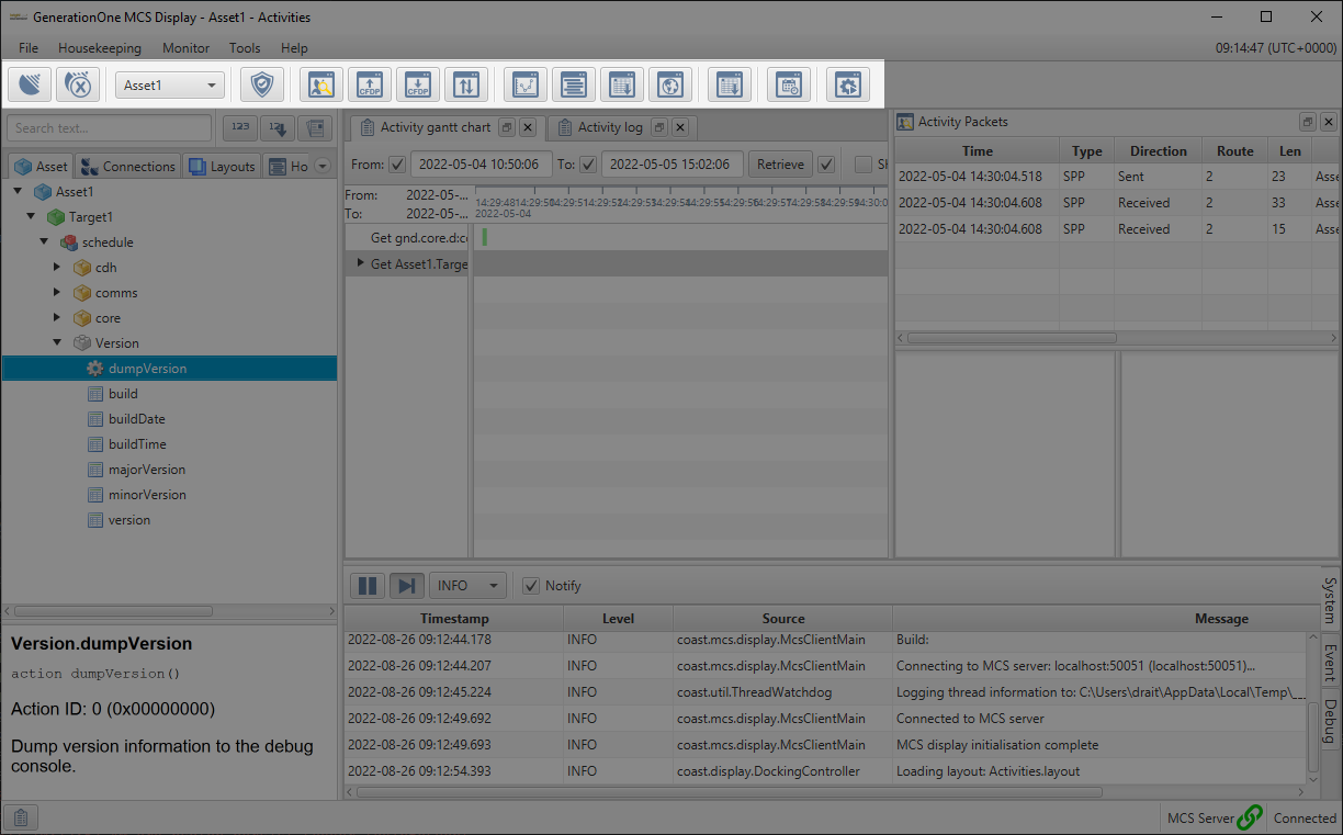
The asset dropdown allows you to select an asset to view. Other functions operate in the context of the currently selected asset.
The buttons on the toolbar, listed in Toolbar buttons with equivalent menu items., provide shortcuts for commonly-used menu items. Most of them provide access to dockable views that allow you to integrate with the spacecraft in various ways. Hover over them to see their tooltip description.
| Icon | Menu item | Function |
|---|---|---|
|
File → Connect |
shows the connection dialog |
|
File → Disconnect |
disconnects all connections to the current asset |
|
Housekeeping → Check housekeeping |
enables or disables checks for housekeeping with check violations appearing in the log view |
|
Monitor → Packet monitor |
displays the packet monitor view |
|
Monitor → CFDP uplink |
displays the CFDP uplink dialog |
|
Monitor → CFDP downlink |
displays the CFDP downlink dialog |
|
Monitor → Transfers |
displays active transfers both downlinks and uplinks |
|
Monitor → Graphs |
opens a graph view that displays parameter values in a graph |
|
Monitor → Parameter table |
opens a parameter table that shows the last known parameter value in a table |
|
Monitor → Parameter log |
opens a parameter log; a time based view of parameter values |
|
Monitor → Map |
displays the map view |
|
Monitor → Event log |
opens an event log that shows a time based view of event details |
|
Monitor → Time-based schedule |
shows the ground schedule view to administer the MCS’s ground schedule |
|
Monitor → Script execution |
shows the interface for executing preconfigured scripts |


2.3. Mission explorer
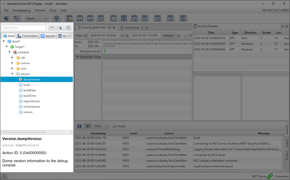
The left-most panel of the user interface is the mission explorer. This is a tabbed explorer containing the items associated with the current mission, which can be seen in Figure 4, as a tree view.
The text field above the explorer tabs allows you to search for and navigate to items in the asset component structure by name. The leftmost button toggles the display of numerical identifiers for items in the structure, useful as inputs to some fields. The middle button sorts the various trees according to these identifiers. The rightmost button toggles the documentation pane on/off.
The asset tab is initialised using a spacecraft database (SCDB), and displays the component structure of the currently-selected asset. More information on setting this up can be found in Section 3. When the MCS is connected to the asset, you can access on-board parameter values and actions by double-clicking on their entries in the explorer. This is explained in more detail in the following chapters.
The Connections tab shows the saved connection configurations. These may be for connections through third-party Ground Station Networks, or through direct connections.
The Layouts tab shows the saved layout configurations. A layout stores all data relating to the current state of the user interface, allowing you to switch seamlessly between different workflows.
The Housekeeping tab shows the housekeeping definitions currently associated with the MCS: aggregations and aggregation-beacon mappings. An aggregation defines data packages which are regularly received and decoded by the MCS. The mapping tells the spacecraft what aggregation to send using which beacon.
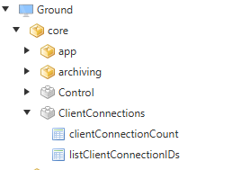
The Ground tab shows parameters and actions defined in the MCS itself, including communication statistics and settings relating to the currently selected asset, as well as synthetic parameters, extensively detailed in Section 18. The Ground tab also displays details of current MCS client connections (Figure 5). The clientConnectionCount parameter reflects the number of MCS Display clients which are currently connected to the MCS Server, and listClientConnectionIds returns a list of client connection identifiers.
| Each time an MCS Display client connects to the MCS Server, the Server allocates a new connection identifier for that connection. This is based on the system username and hostname supplied by the client, together with the date and time of connection. This identifier is included in the Activity Log (see Section 4.7) for any Parameter Get and Set operations and Action Invoke operations initiated by a display client. |
| The allocation of client host names and usernames is the responsibility of the customer’s IT administration. |
The bottom section of the Mission explorer displays the documentation for the currently selected element. This includes the short name of the element, the fully qualified name, action ID, and any description available. It can be displayed/hidden using the rightmost button next to the search bar above the tabbed panel.
2.4. Docking area
The remaining upper right area, shown in Figure 6, is the docking area.
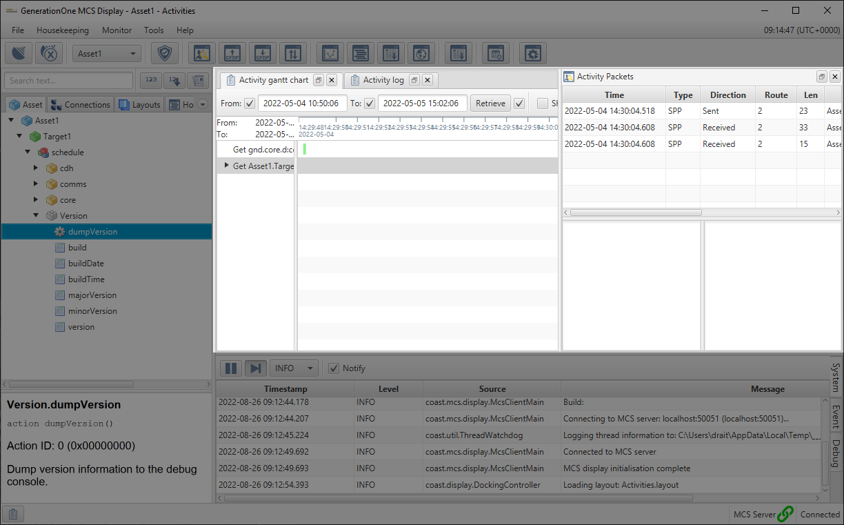
This is a configurable view that you can change and modify depending on the task at hand. For example, this view could contain a window to interact with a component’s parameter, a window to invoke a component’s action, a window to see ongoing file transfers or any of the other various possibilities. This area allows you to customise a unique layout that can be geared to your particular use of the MCS.
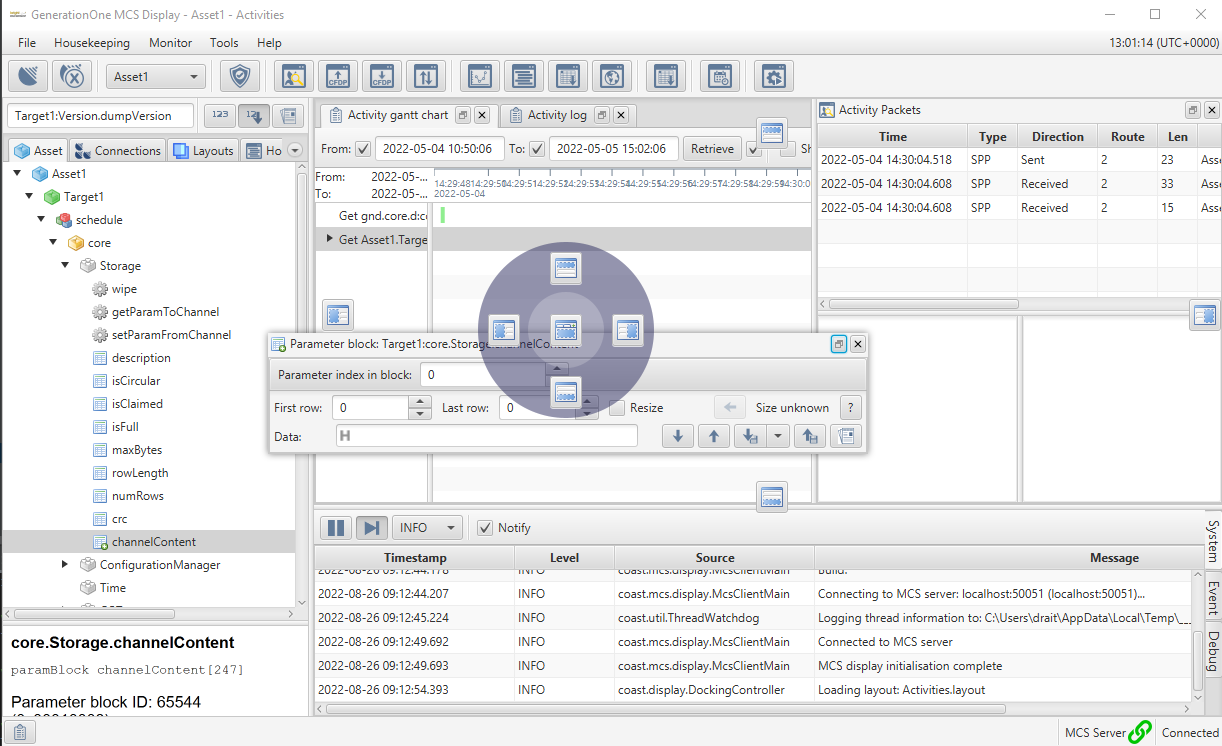
When you first open a dockable view they will float as separate windows. Add a window to the current layout by dragging it over this area and dropping it on one of the drop destination symbols, as in Figure 7.
To dock a view as a split window drag the component into one of the four edge handles. The circular control represents the currently hovered window whilst the outer edge handles represent the whole window.
To create a tab view drag a floating dock view into the centre handle.
To undock a window and turn it back to a floating window drag the title bar of a docked view to anywhere on the screen or click the unmaximise button in the corner of the view.
Floating windows can be docked together themselves, using the same approach described above, to create more complex floating views.
2.5. Layouts
Your layout is described by the current arrangement of windows, docked panels, window sizes and the internal state of various controls in the display. When you initially load the MCS the default layout will be used by the MCS. Subsequent layout changes will be saved when closing the MCS or switching layouts (assuming the current layout is not locked).
You may want to consider using an alternative layout depending on what task you’re trying to achieve. To do this simply right-click the layouts node in the mission explorer and choose ‘New’, pick a name and click OK. Make changes to the current layout and either right click the node and press save or simply exit the MCS.
The layouts tab in the mission explorer shows the available layouts in the MCS – initially this will just be the default layout. Double-clicking or right-clicking and choosing open on these nodes will swap your layout to this new layout saving the old one.
| The context menu of a layout will give you more options for modifying a layout such as deleting, renaming or duplicating. |
2.5.1. Locking layouts
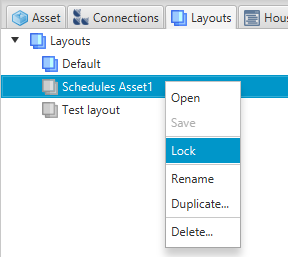
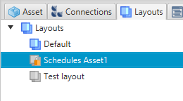
The option to save an old layout is important because sometimes you may have a template layout that you don’t want changed. To prevent this happening you must lock the layout by right-clicking a layout node and clicking lock (Figure 8), note the padlock icon on the layout node that appears (Figure 9). This will prevent the layout from being modified from anything other than its current state.
2.6. Log view
At the bottom right of the main MCS Display, highlighted in Figure 10, is the log view. This is where any system, spacecraft, or OBSW debug events are displayed.

The log view displays logs from 3 sources, each displayed in their own tab:
-
System logs – logs originating from the MCS itself. These could be anything from the failure of a connection to reports on how the ground schedule is being executed. If the behaviour of the MCS is amiss the first place to look would be the system logs.
-
Event logs – this tab shows events originating from the OBSW. This will be tied to a particular on-board component
-
Debug logs – these logs show debug information specific to the OBSW. These logs should show data at a higher level of detail than the event log.
The pause button temporarily suspends updates to the current log view. Un-pausing will resynchronise any missing logs whilst it was paused and allow further updates to the log view. To ensure that updates are always visible, click the auto-scroll button to the right of the pause button. This will auto-scroll the log view to the bottom when additions are made to the log.
You can configure the log display level using the dropdown in the toolbar. This filters out logs which are below the selected severity level. The "Notify" checkbox will cause the relevant tab to flash or blink whenever updates are made to the log. Unchecking this will disable notifications and display a small warning icon in the tab.
The logs here are archived. You can scroll through into the archive by scrolling up through the local logs with your mouse wheel until you hit the top. Once at the top the MCS will start pulling logs from the archive, extending the available scrolling height and date range.
2.7. Status bar
The status bar at the foot of the display shows the status of current tasks, as in Figure 11. This is only displayed while the task is active. The status of completed tasks can be displayed in the Active Tasks view (see Section 4.6), which can be opened using the button at the left of the status bar.
In the right-hand corner, the status bar also displays the status of two connections: the MCS Display’s connection to the MCS Server, and the MCS Server’s connection to an asset. These will both show green symbols when connected.

3. Getting Started
This section provides you with practical guidance on how to use the MCS. It will get you connected to the OBSW and allow you to interact with the spacecraft through the different GUI components. To connect the MCS to the onboard software you will first need to set up the MCS to match both your deployment and the ground equipment used to connect to it.
3.1. Mission Management
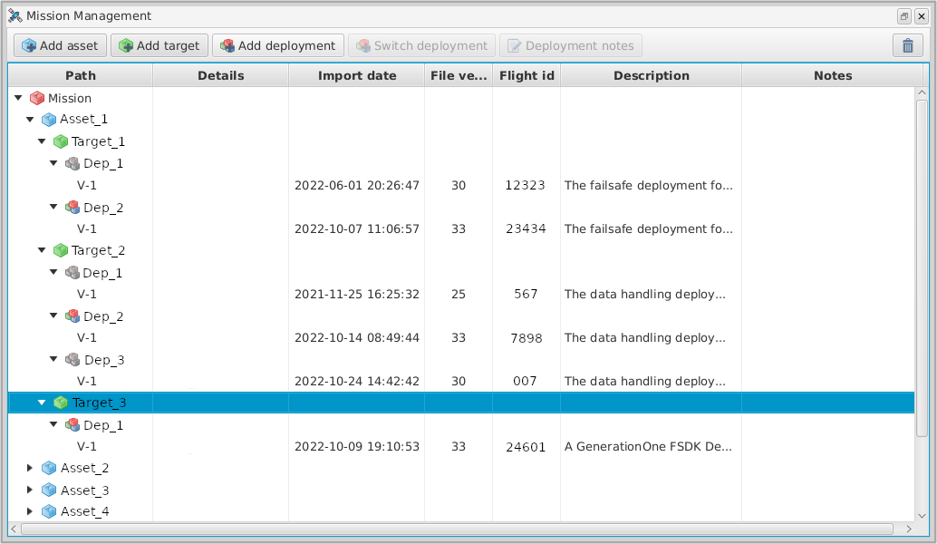
In order to efficiently manage your spacecraft, a few concepts must be introduced which are crucial to understanding and operating the MCS: missions, assets, targets and deployments. Most users will have some intuitive understanding of these from operational experience, but in the interest of wider accessibility, they will be explicitly discussed here. Throughout this explanation Figure 12 will be referred to. This shows the mission management window accessible through File → Mission Management, with some assets, targets and deployments loaded.
3.1.1. Mission
A mission refers collectively to all the objectives that are being attempted and the resources required for them. This involves all the available satellites, OBSWs, and any other resources. A mission should have clear goals and a way to meet them, determined during the planning stage.
In MCS terms, a mission is the single overarching framework in which everything will be defined. It is not possible to have multiple missions in one instance of the MCS. It isn’t necessary to add or remove them - it will start with a default mission. In Figure 12, the mission can be seen at the top of the "Path" column on the left, represented by a red box symbol.
3.1.2. Asset
An asset is a representation of the physical object which we are attempting to reach and control. It has hardware and software that can be used to talk to it. In most cases in the MCS, an asset is a satellite. Assets are represented in the MCS by a blue box symbol. They must have at least one target associated with them in order to be able to perform any functions.
It is possible to have multiple assets in the same mission, each with their own distinct targets and configurations, as seen in Figure 12 named Asset_1, Asset_2, Asset_3 and Asset_4. A new asset can be added by clicking the Add asset button, leftmost in the row of buttons at the top of the window. This will open a pop-up window in which you can specify the asset name. Asset names must be unique, and the MCS will reject duplicate asset names.
Selecting an asset and pressing the trashcan button, at the right-hand side of the aforementioned row of buttons, deletes it through a confirmation dialog.
3.1.3. Target
A target is the specific part of an asset that we are trying to talk to. This is usually an on-board computer running some flight software. Targets are represented by a green box in the mission management system. Targets must have at least one deployment associated with them in order to be contactable.
It is also possible to have multiple targets on an asset. In Figure 12, there are three targets on Asset_1: Target_1, Target_2, Target_3. Each other asset, collapsed on the display, also has its own target(s). A new target can be added by selecting an asset and clicking the Add target button in the row of buttons at the top of the window. Names of targets must be unique for the same asset, with duplicate names rejected. However, it is acceptable to use the same target name for two different assets.
Selecting a target and pressing the same trashcan button deletes that target in the same way as for an asset.
3.1.4. Deployment
A deployment is fundamentally a definition of the spacecraft systems, which holds details of the OBSW on a particular spacecraft. Examples of such details are the unique identifiers of the components, how they are interconnected, how they are initialised, managed and configured. It also specifies how to access their constituent parts, known as parameters and actions. The flight side software will have a deployment active on it. On the ground side, deployments are contained in SCDBs. A target must have at least one deployment associated with it, represented by the three-box symbol in Figure 12, either multicoloured or grey. When multiple deployments are associated with a single target, only one can be in use at a particular time. A coloured symbol indicates that a deployment is currently active, while a grey symbol indicates that it is not.
Selecting a target and clicking the Add deployment button in the row of buttons brings up the dialog shown in Figure 13. Of the six user-input fields that are shown, two are mandatory:
-
Deployment ID:The name that the deployment will have in the MCS. -
Definition file:The SCDB file which holds the deployment. Clicking the ellipsis button to the right of the field will bring up a file explorer, allowing you to navigate to and select the correct file.
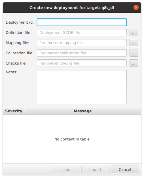
There are four further optional fields: Mapping file:, Calibration file:, Checks File:, and Notes. The first three of these are file inputs for calibrations and checks, discussed further in Section 10. Clicking the ellipsis button to their right again opens the file explorer for you to select the correct file. The Notes field can hold any comments the user might have on a particular deployment, which will be displayed in the Notes column seen in Figure 12.
There are three buttons at the bottom of this window: Load, Import and Cancel. When at least a deployment ID and a suitable SCDB file have been specified, the Load button will become active.
Make sure you fill out the other fields of the import dialog if they are required before clicking Load.
|
Clicking this performs basic verification checks on the SCDB and other specified files. If any errors are found, they will be displayed in the bottom of the window under the Message column, otherwise only informational or warning messages will be displayed. Any errors must be read and resolved before clicking the Import button to add the deployment. This will initialise and populate the mission explorer.
When a deployment is selected, a new button will appear on the row seen in Figure 12 labelled Update deployment. This allows you to keep the current name and target for the selected deployment, but specify new files and notes for it.
If multiple deployments have been associated with a target, only one can be active at a time. This can be changed by selecting a deployment and clicking Switch deployment on the buttons row of Figure 12. This will activate the selected deployment and de-activate the currently active one. For a target with a single deployment, this button does not action any changes.
To summarise: in setting up the MCS you will have to configure an asset, target and a deployment. An example of an asset is a satellite, so a target in this instance would be a computer on the asset that runs a specific deployment. On the ground side, a deployment is represented using an SCDB file.
-
Navigate to File → Manage Mission to get to the mission Management view.
-
Add a new asset and a target for the asset with unique names. Then add a deployment to the target by selecting it and clicking
Add deployment. -
This will bring up a new window where you can give the deployment an ID and point the
Definition fileparameter towards your SCDB file. First load the deployment, which will perform some verifications on it, then import it. This will initialise the mission explorer tree. -
Explore the tree to familiarise yourself and ensure that the expected components are visible for this mission.
3.2. Connections
3.2.1. Set up the MCS for the ground equipment
The next step is to connect the MCS to the OBSW. In order to do this, you must create a connection point, which will appear in the mission explorer Connections tab. This can represent a direct connection (e.g. Serial link, TCP Client or Server) or a Ground Station Network. connection points are saved as part of the MCS mission configuration. They allow connection configurations (protocol, address, port, etc.) to be saved as named items which can be used to connect to assets.
An existing connection point can be edited when there are no live connections using it, by right-clicking on it and selecting the Configure option.
|
To enable connections via a third-party Ground Station Network, use the context menu entry in Ground Station Networks to add the required details for the desired third-party network. A different menu option will be displayed, and a different configuration dialog will be presented, for each supported network type. Section 16 gives details of how to configure the system to use the third-party networks supported natively by MCS.
To create a connection point for direct connections using TCP, UDP or other protocols, follow these steps:
-
Right-click on the
Directitem in the mission explorer tree to access its context menu, and selectAdd direct connection. -
Enter a valid, unique name for the connection point. This must begin with a letter, and must only contain letters, digits and/or underscores.
-
Select the communication protocol in the dropdown selector.
-
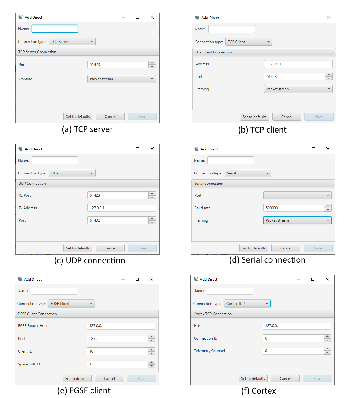
Configure the connection settings with the appropriate details. For TCP this is usually the IP and port of the computer that the OBSW is running on. In some cases you’ll want to run the MCS as a server instance and the OBSW should act as a client, connecting when it starts. To do this use the drop-down to select TCP server and choose an open port. Examples of connection configuration dialogs can be seen in Figure 14.
-
The
Savebutton should become enabled when you enter a value in the name field. When you save the configuration, it should be displayed as a new item in the mission explorer tree. If required, the configuration can be edited via the context menu for that item, whenever it has no active connections.
Connection Point Groups
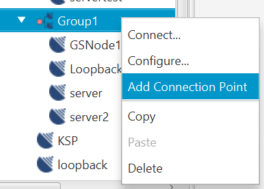
Direct connection points can be created in groups, allowing you to connect to or disconnect from the current asset via multiple direct connection points in a single operation. To create a group, select the Add Group… option from the direct connection points node in the mission explorer. Add individual connection points to the group using the Add connection point option on the group’s explorer node (see Figure 15).
When adding or updating a connection point within a group, an additional checkbox in the configuration dialog sets that connection point as the preferred uplink connection point when connecting via the group’s Connect menu option.
You can copy connection points or groups, or move connection points into, out of or between groups, using the Cut/Copy/Paste context menu options. If moving a connection point creates a name conflict, you will be prompted for a new name when you select the Paste option.
|
Asset Restrictions
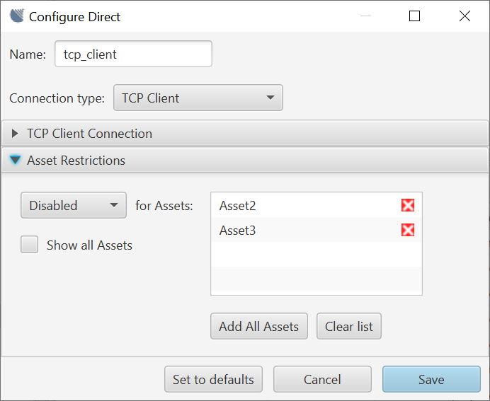
By default, a new connection point can be used to connect to any asset. However, where a connection point or group is intended for use only with selected assets, it can be configured to prevent its use with other assets. These restrictions can be applied to connection point groups, and to any individual connection points which are not in a group. Figure 16 shows the asset restrictions configuration display for a direct connection point. (The restrictions are displayed in a collapsible pane below the connection type settings for the connection point.)
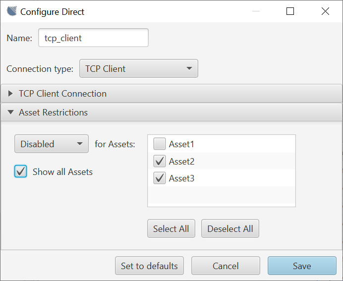
The selected assets list is initially empty, meaning that no assets are disabled. This means that the connection point will also be enabled for any newly created assets which are not added to the list. If the configuration is updated to make the connection point Enabled only for selected assets, then the connection point will be disabled for any new assets, until they are added to the selection. Individual assets can be added to the selected list by switching to the All Assets list view (Figure 17) and selecting the checkboxes for the assets to be added.
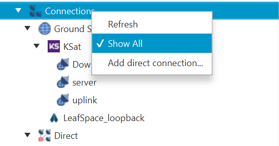
By default, the mission explorer only displays connection points which are enabled for the current asset. To remove this filter, select the Show All option in the connections root node (Figure 18).
|
Automatic Reconnection
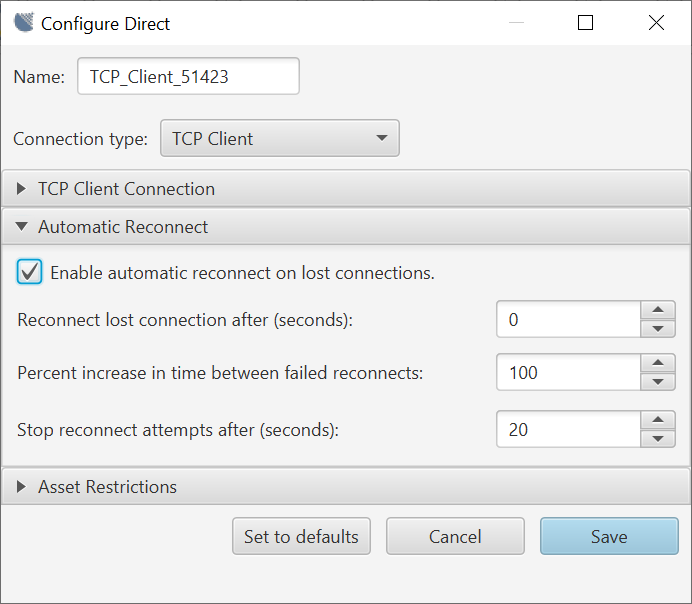
Connection points can be configured to reconnect automatically when MCS detects a loss of connection. Where applicable, the Automatic Reconnect settings can be updated via the connection point configuration display, as shown in Figure 19.
3.2.2. Connect the MCS to the OBSW
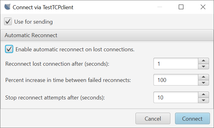
Once a connection point has been created, you can connect to the current asset by right-clicking the connection point (or connection point group) in the explorer, and selecting Connect. Alternatively, you can click the Connect button in the toolbar and select the connection point (or group) from the dropdown list. Deselect the Use for sending option if the connection is not to be used to send telecommands. When connecting manually via a direct connection point, you can override its automatic reconnect settings via the dialog seen in Figure 20.
If the connection is successful, an entry with a satellite icon labelled with the asset name will appear under the connection point item in the mission explorer tree. If running as a TCP server, the MCS will now be listening for connections on the port specified. The OBSW should establish a connection, and the status in the bottom right corner of the MCS should reflect this.
| The direction of transmission in each connection is indicated by one or two arrow symbols beside the asset name, indicating upward (to the satellite), downward, and bidirectional connections. |
You can open simultaneous connections to a given asset via multiple connection points (for example: one for sending telecommands, and another for receiving telemetry data). Only one connection per asset can be designated for sending data at any time, so selecting Use for sending on a new connection will clear that marker on any existing live connections to the same asset. To select an existing connection to be used for sending, right-click on the connection satellite icon in the explorer tree and select the Use for sending option.
To close a connection, right-click on the connection entry in the explorer and select Disconnect in the context menu. To close all connections to the current asset via a connection point group, select the Disconnect from <Asset> option on the group entry. Alternatively, all connections to the current asset can be closed by clicking the Disconnect button in the toolbar.
3.2.3. Protocol Properties
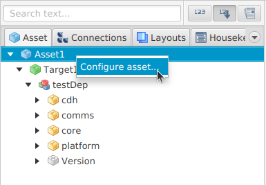
The protocol properties for the current asset can be viewed and updated via the File menu, or the Configure asset… context menu item for the asset entry in the mission explorer tree (Figure 21). This section describes the different options available in the protocol properties window and is organised into tables according to the different sections in the window.
Different protocol properties can be specified at either an asset or a target level. If a protocol property is specified at the target level, it means that each target in the asset can use the property differently, and if the property has a value then the value specified will only be applied to the target selected. Switching between assets and targets can be done using the dropdown shown in Figure 22.
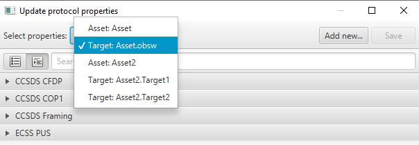
In the dropdown menu, the assets/targets are pre-fixed with either 'Asset' or 'Target' so it is explicit what is being selected.
Asset Protocol Properties
| Property | Description |
|---|---|
Use AX25 on uplink |
Set to true to enable AX25 uplink framing support |
AX25 uplink has start flag |
Set to true to enable AX25 uplink start |
AX25 uplink has end flag |
Set to true to enable AX25 uplink end flag field |
AX25 uplink has FCS |
Set to true to enable AX25 uplink FCS field |
Use AX25 on downlink |
Set to true to enable AX25 downlink framing support |
AX25 downlink has start flag |
Set to true to enable AX25 downlink start flag field |
AX25 downlink has end flag |
Set to true to enable AX25 downlink end flag field |
AX25 downlink has FCS |
Set to true to enable AX25 downlink FCS field |
AX25 Local callsign |
The AX25 callsign used in the ground software |
AX25 Remote callsign |
The AX25 callsign used by the remote entity |
AX25 Local SSID |
The AX25 SSID used in the ground software |
AX25 Remote SSID |
The AX25 SSID used by the remote entity |
| Property | Description |
|---|---|
FOP1 Sliding width window |
Sets how many frames to send in a window |
T1 initial |
Sets what the round-trip time is, so how long to wait before re-transmitting |
Transmission limit |
How many times to retry transmitting |
| Property | Description |
|---|---|
Use CCSDS datalink for TC |
Set to true to use CCSDS SDLS framing up |
Use CCSDS datalink for TM |
Set to true to use CCSDS SDLS framing down |
Use CCSDS datalink security |
Set to true to enable security in CCSDS SDLS framing |
TM Transfer Frame length |
The size in bytes of a CCSDS TM frame |
TC Transfer Frame length |
The size in bytes of a CCSDS TC frame |
TC Virtual Channel ID |
The Virtual Channel ID to insert in the header of a CCSDS TC frame |
TM Virtual Channel ID |
A list of Virtual Channel IDs of the TM SDL protocol to receive telemetry |
Include segment header in TC frame |
Set to true if segment header is included in TC frames |
Include Frame Error Control Field in TC frame |
Set to true if Frame Error Control Field is included in TC frames |
Include Frame Error Control Field in TM frame |
Set to true if Frame Error Control Field is included in TM frames |
Discard TM Frames on Error Control failure |
Set to true to discard TM frames with a CRC failure |
| Property | Description |
|---|---|
Use CCSDS TC Sync & Coding |
Set to true to use |
Use CCSDS TM Sync & Coding |
Set to true to use |
Block Interleave Depth |
The number of code blocks that are in a single Channel Access Data Unit, will default to '1' if not set |
| Property | Description |
|---|---|
PUS Default Target |
Set a default target to use for PUS |
| Property | Description |
|---|---|
Accent colour |
Set the asset to have a colour scheme to use within the MCS |
Inhibit uplink |
Set to true to inhibit any transmission |
Spacecraft ID |
Used by CCSDS framing |
NORAD ID |
Required by LeafSpace Ground Station Network |
Uplink Frequency (Hz) |
Used by LeafSpace Ground Station Network |
Downlink Frequency (Hz) |
Used by LeafSpace Ground Station Network |
| Property | Description |
|---|---|
Use HMAC authentication |
Set to true to enable HMAC authentication |
HMAC key |
The hex of the HMAC authentication key |
| Property | Description |
|---|---|
Use SwissCube data layer |
Set to true to enable SwissCube downlink framing |
Target Protocol Properties
| Property | Description |
|---|---|
CFDP APID |
The CCSDS APID to use for CCSDS CFDP transfers |
CFDP RX APIDs |
The CCSDS 'Receive' APID to use for CCSDS CFDP transfers |
CFDP Local Entity Id |
The CCSDS CFDP entity id for ground |
CFDP Ack Timeout |
The timeout for sending an Ack/Nack (in ms) |
CFDP PDU transmit gap |
The gap to wait between sending CCSDS CFDP file parts (in ms) |
CFDP PDU size |
The size in bytes of a CCSDS CFDP PDU |
CFDP Ack limit |
The number of ack/nack retries before timing out a CFDP transfer |
| Property | Description |
|---|---|
Use CCSDS COP1 |
Set true to use CCSDS COP1 for the selected target |
| Property | Description |
|---|---|
TC Virtual Channel ID |
Set a different Virtual Channel ID for TCs per-target |
| Property | Description |
|---|---|
PUS C |
Set to true to use PUS-C rather than PUS-A |
PUS APID |
The CCSDS APID to use for ECSS PUS services |
PUS TM Time coarse bits |
The number of coarse time bits in a ECSS PUS packet |
PUS TM Time fine bits |
The number of fine time bits in a ECSS PUS packet |
3.2.4. Managing CCSDS COP1
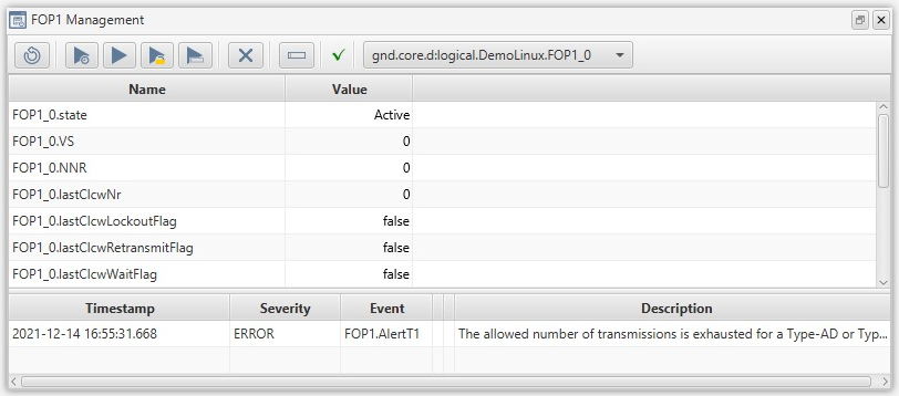
The MCS provides a basic administration panel for observing the internal COP1/FOP1 process and controlling its behaviour. Basic information on the state of the remote FARM1 process as received from the flight software can be examined, as seen in Figure 23. It allows the operator to monitor and control the state of the ground FOP1 process.
As startup FOP1 process will be in the Initial state in which all TC frames will be transmitted in BD mode. To move to the Active state one of the four start buttons should be actioned from the GUI toolbar (which one depends on the desired start mode and current state of the remote FARM1 process). To stop the use of the COP1 process the X button should be used which will return the state back to Initial.
| For more information about the COP1 specification, see the CCSDS 232.1-B-2 blue book. |
3.2.5. Test the connection to the OBSW by retrieving a component’s parameter
-
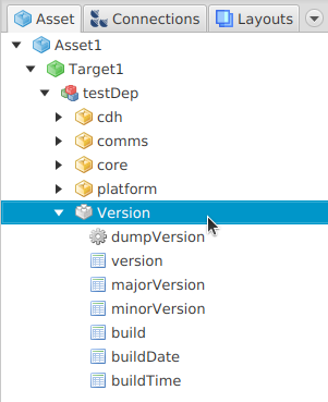
To retrieve a component parameter, expand the version component in the mission explorer (Figure 24) and double-click the version parameter. The parameter window should display.
-
Click the downwards arrow to retrieve the component parameter’s value. You should see the get request complete at the bottom left of the status bar. If the steps were successful, the data text field should show the contents of the parameter.
3.3. Interacting with the OBSW
This section goes into more detail on the fundamental interactions that you’ll be making with the OBSW through the MCS.
3.3.1. Interacting with parameters
One of the most fundamental ways of interacting with Bright Ascension’s onboard software is through the setting and getting of onboard parameters. Parameters hold the current state of an onboard component and manipulating this state is fundamental for command and control of the spacecraft.
Parameters may be read-write or read-only. Double-clicking a read-write parameter from the mission explorer will show the parameter view, as in Figure 25.

The following parameter actions are available:

|
Get the contents of the parameter. Display it in the data field if successful. |

|
Set the contents of the data field as the parameter value. |

|
Similar to set and get. However, a large downlink/uplink to the parameter will be initiated, for large amounts of data. The appropriate protocol according to the configuration will be used by default. |

|
Show the associated documentation for this element. |
The arrow to the right of the large data downlink button allows you to choose between downlinking the data to a single file, or to multiple files. It also allows you to manually choose a protocol, if the default choice is unsuitable. Choosing the multiple file option will then prompt the user for the number of rows of the parameter to be put in each file.
Read-only parameters have a similar display to the above, shown in Figure 26. However, the set buttons will be greyed out, as the set function is unavailable. The get function and documentation work the same as above.

The initial data encoding mode is dependent on the type of parameter. To change this, click on the letter to the left of the data text fields contents. Depending on the parameter the data will be encoded depending on the following types:
-
H - Hexadecimal
-
D - Decimal
-
B - Binary
-
S - String
-
R - Real (floating point)
| The selected data encoding modes and values in parameter views are stored as part of the current layout, so they will be restored when reloading that layout. Therefore, the displayed value may not reflect the current value of a parameter, but rather the value which will be set on clicking the upwards arrow button. This allows multiple parameter values to be stored in a layout, so that the user can quickly set up a known configuration by loading the layout and performing set operations on the displayed values. |
3.3.2. Interacting with multi-row parameters
Multi row parameters are functionally vector parameters that are defined in the on-board software. They can store multiple values, all the same type, with one value on each row as a more efficient way of storing data. Multi row parameters can be administered in the same way as single or fixed parameters. The only difference is that you’ll need to specify a row range via the fields above the data field in Figure 27.

The first and last row fields specify the range to get or set. The resize checkbox behaves slightly differently depending on whether it’s a get or a set. For a get when the resize flag is set the requested index range will be resized to fit the number of rows. For example if the parameter contains 3 rows and you request a range of 0 to 50, rather than fail, the get operation will return all 3 rows. The request has been resized to fit the available rows. When setting a parameter the resize flag, controlled via the related checkbox, will change the number of rows available effectively downsizing the rows to fit the set operation.
The ? and left arrow buttons act to query and then set the number of rows on a parameter respectively. Clicking the ? will perform a query to get the number of rows currently held by this parameter. This will display to the left of the button. Pressing the left arrow will set this value to the last row effectively binding the limit of the number of rows set to the current parameter row size. This is useful for setting all rows without resizing.
3.3.3. Invoking actions
The other fundamental way of interacting with onboard components is through action invocations. Actions perform some operation on/with a component and have the option of adding arguments. To invoke an action double click it from the mission explorer to display an invoke action window as in Figure 28, which will provide a dockable view for that action in the OBSW. The title bar of the view contains the fully qualified name of the action. Pressing the invoke button, denoted by the right arrow, invokes the action.

If the action requires an argument then the argument entry field will be available and the invoke button will be greyed out until a valid value is supplied. The argument field can be switched between the value entry modes by clicking on the small letter at the beginning of the argument entry field. Valid modes are:
-
H - Hexadecimal
-
S - ASCII encoded string
| As with the parameter view, the documentation for the action is accessible as a pop out display using the button to the right of the invoke button. |
3.3.4. Managing the on-board file system
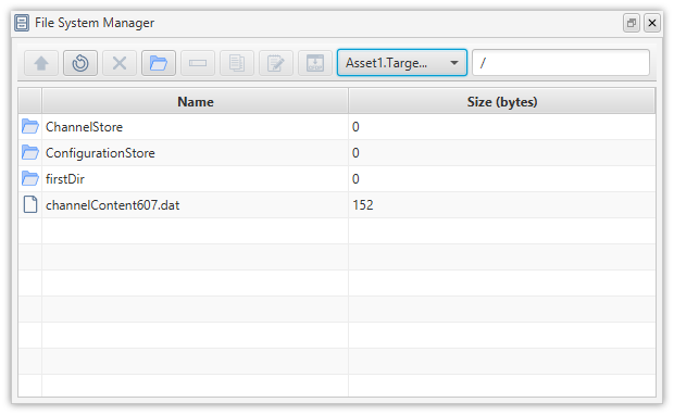
The MCS provides support for the FileSystemManager on-board component. It allows you to perform basic file operations using a file manager similar to most operating systems. This avoids the need to manage files using parameter manipulation and action invocation. The File manager view will do the component manipulation for you.
To access the File manager view, find a currently-connected asset’s FileSystemManager component in the mission explorer, right click and choose Explore. The File manager view will initialise to the root directory, as seen in Figure 29. To display the contents of the directory, press the refresh button or press F5.
A number of actions are available:
-
To create a directory click the button with the directory icon.
-
You can navigate the directories by double clicking or pressing enter when a directory is selected.
-
You can copy and paste directories or files using ctrl+c and ctrl+v.
-
Files can be deleted by pressing the ‘X’ button on screen or delete on the keyboard. Directories can only be deleted if the directory itself is empty.
-
You can rename using the button with the text field icon or by pressing the F2 key whilst a file is selected.
-
You can navigate up by pressing the up button or by pressing ctrl+up.
4. Monitoring
Monitoring telemetry is an integral part of operating a spacecraft. This chapter describes the various ways you can monitor the spacecraft and present the data.
4.1. Packet monitor
The packet monitor, seen in Figure 30, shows telemetry and telecommands at the packet level. This is a good way of getting a picture of what is currently flowing between you and the spacecraft. It can be accessed from the toolbar button highlighted in Figure 31.
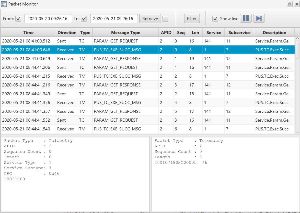

The pause button prevents further input from the current link. Unpausing will synchronise the telemetry to the latest and allow further updates. The autoscroll button will autoscroll output keeping the view matched to the latest data. The From and To date range options allows you to filter the displayed packets by date.
4.2. Parameter table
The parameter table displays values of parameters in tabular form, showing the raw as well as its calibrated value, if it has one, as in Figure 32. Its toolbar button is highlighted in Figure 33.
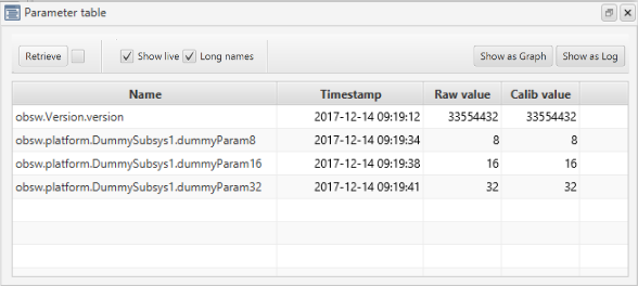

The displayed parameters can be chosen by dragging and dropping parameters from the mission explorer into the table. The long names checkbox indicates whether to use the fully qualified parameter name. The Show as Graph and Show as Log buttons will export the parameters viewed here to the respective view. See their sections in this chapter for more detail. The Show live checkbox allows for live updates in the window.
4.3. Parameter log
The parameter log displays a historical log of parameter values (Figure 34), and can also be accessed from the toolbar (Figure 35). Rows indicate values retrieved from the chosen parameters, in ascending time order. The first column is the update time and the following columns represent the values of the chosen parameters.
To choose parameters, simply drag and drop parameters from the mission explorer. Alternatively you can display the set of parameters that make up an Aggregation as a Parameter Log by right-clicking the Aggregation under the Housekeeping node of the Mission Explorer and choosing Open Log. When adding multi-row parameters via drag and drop a dialog will be displayed indicating which rows you wish to add. This dialog acts in the same way as double-clicking a multi-row parameter.
To remove parameters, right-click on the table and use the remove menu, or hit delete on the keyboard.
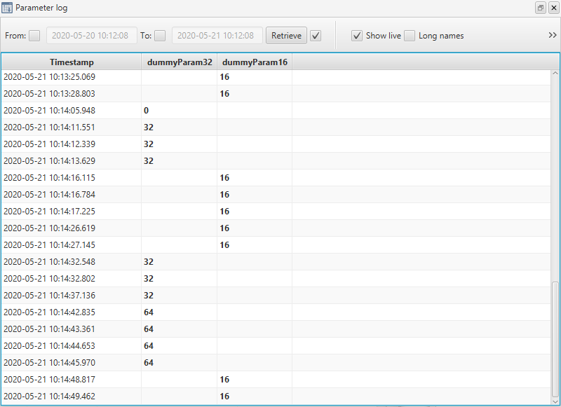

Two considerations must be made when looking at the values in a parameter log:
-
The last value does not necessarily represent the current value, owing to the fact that state may have changed on the flight side. This won’t be updated on the ground side as it happens. An update is guaranteed whenever the MCS receives a parameter value.
-
If two or more parameters are displayed and an update arrives for just one of the parameters, the log view will display the updated value for the updated parameter and the last known value for the other parameter.
To differentiate which parameter has updated, the value is highlighted in bold.
The time selection controls at the top allow you to configure a time range to retrieve from the archive. To ensure real-time updates to the parameter log, tick the Latest checkbox. Looking further to the right of the toolbar you’ll find the Show long names checkbox; this will display the fully qualified parameter names for the column headers just like with other views.
The Show calibrated values checkbox will swap all the values to their calibrated values (see Section 10.1 for further details on how to set up calibrations). If they don’t have a calibrated value, the value will remain as the raw value.
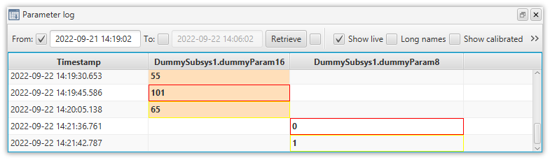
Finally, if the Highlight check results checkbox is selected, the results of checks (Section 10.2) are reflected by the background and border colouring in each value’s table cell, as described in Parameter check result indicators.
| Check | Warning | Error |
|---|---|---|
Raw value |
Yellow border |
Red border |
Calibrated value |
Amber background |
Red background |
In the example in Figure 36, the 2nd entry indicates an ERROR check result for the raw value, and a WARNING for the calibrated value, and the last two entries indicate only ERROR and WARNING raw value check results.
4.4. Graph view
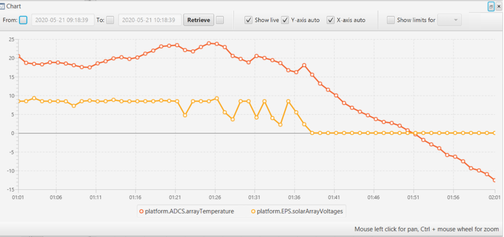
The graph view plots parameter values on the y-axis of a graph, with the x-axis indicating time. This is directly equivalent to the parameter log view but the data is plotted graphically. An example of such a graph can be seen in Figure 37. It can also be accessed from the toolbar, via the button highlighted in Figure 38.
To add a parameter to a graph from the parameter log, right-click on the parameter and choose Open in graph. You can also plot the values of parameters by dragging a parameter from the Mission explorer into the chart view. There is no limit on the number of parameters that can be dragged and dropped into the view, and plotted simultaneously. For aggregated housekeeping definitions, right-click an Aggregation node in the Mission Explorer’s Housekeeping tab, and choose Open graph… to display a graph of all the parameters contained in the aggregation. To delete parameters from the view, right click anywhere in the graph, choose delete and select the parameter to remove from the chart.
You can navigate the chart by panning and zooming. To pan the view drag the left mouse button in the chart area. To zoom the chart, hold control and scroll the mouse wheel in or out.
X-axis auto and Y-axis auto checkboxes allow you to fit the graph to the current range of data ensuring the maximum and minimum values are within the bounds of the graph.

| Ticking the date range boxes will limit any archived data retrieved to the specified date range. |
4.5. Map display
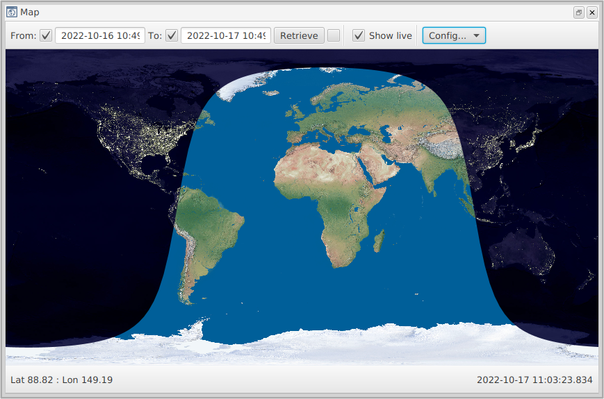
The map display can show the path of multiple space objects against the earth in a 2D view. It can also display visibilities to configured ground stations, a list of which must be given to the MCS for plotting (see Section 11.2 for details on how to place ground station locations into the correct configuration file for the MCS). The basic display is seen in Figure 39. It can also be accessed from the toolbar button highlighted in Figure 40.

There are two modes of configuration available: live or historic mode. Live mode has the Show live checkbox ticked, as in Figure 39, and will update itself so that you can see the ground trace as it happens. Historic mode, when this checkbox is unticked, will only show historic logged data between the dates and times specified in the From: and To: fields.
Configuration of the map display is done through the Config… dropdown. A series of display options are available:
-
The
Stationsoption will show the position of available ground stations when selected. -
Visibilitiesenables visibility footprints around ground stations, which indicate when the satellite will be visible from the ground station. -
The
SpacecraftandTrailsoptions show spacecraft positions and trails on the map display. -
Overlay Landmasshighlights land masses on the map with yellow borders.
Parameters must also be chosen which represent the spacecraft’s logged latitude and longitude. This can be done through Config… → Params…, or alternatively can be imported directly into the MCS via a configuration file as detailed in Section 11.2.
If the display doesn’t look right, the option in the dropdown Params… menu to easily swap latitude and longitude parameters may be useful.
|
4.6. Active tasks view
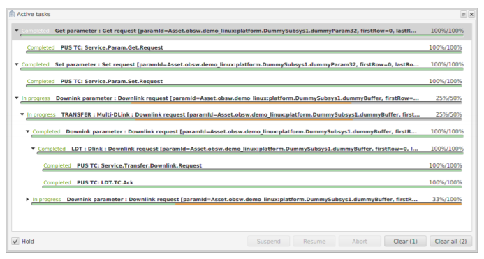
Current activities (e.g. get, set, downlink, uplink, invoke) are displayed in the active tasks view (Figure 41), which can be opened using the button in the bottom left of the main MCS display or via the Monitor → Activities menu option. The nesting of activities indicates parent-child relationships. For example, the top-most activity in Figure 41 was triggered by getting the value of a parameter. This activity then started a PUS get-request to perform the task of asking the on-board software for the value of the parameter.
Each entry in the list details the current state of the activity. These states are:
-
Idle, while the activity is waiting to be started.
-
In-progress, while the activity is running.
-
Completed, if the activity finishes successfully.
-
Timeout, if the activity takes too long to complete.
-
Aborted, if the activity is manually aborted via the
Abortbutton. -
Suspended, if the activity is manually suspended via the
Suspendbutton.
When the Hold checkbox is selected, tasks will remain in the view after they are completed. Buttons allow you to suspend a task, resume a suspended task, abort a task, and clear selected tasks or all tasks from the view.
There are two ways of viewing previously completed activities: the activity log (Section 4.7) or activity Gantt chart (Section 4.8).
4.7. Activity log
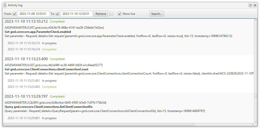
The activity log view (Figure 42) is accessed via the Monitor → Activity log… menu item, and displays activity records retrieved from the Archive.
Parameter Get and Set activities and Action Invoke activities which are initiated from an MCS Display client have a clientId value recorded in their log entries, as shown in the screenshot. This shows the client connection identifier, and you can use the Search function described below to search for activities initiated, for example, by a certain user.
|
The time range for which activities are retrieved and displayed can be set using the From and To fields. The records are retrieved and displayed when the Retrieve button is clicked. If the checkbox beside this button is selected, the records will be automatically retrieved and displayed when this view is opened as part of a saved layout. If the Show live checkbox is selected, new records will be added to the display as they are added to the Archive, so long as the specified date/time range does not exclude the current time.
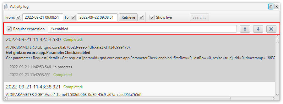
Hitting the Search button displays a search bar in the window, as in Figure 43, which allows you to search for display entries containing a given string. This can be a Java Regex regular expression, if the Regular expression checkbox is selected. Click the arrow keys to go to the next/previous matching entry in the display. When the last matching entry is selected, the search wraps round to the start. The search bar can be hidden using the X button.
Right-clicking on an entry in the view raises a context menu (Figure 44), which gives access to additional views of related archive records.
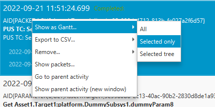
The last two entries only appear when the selected activity was triggered by a parent activity. The first 3 entries in the context menu present the options All, Selected only, and Selected tree. If the Selected tree option is selected, the operation is applied to the selected activity and any child activities triggered by it. Activity log view entry context menu summarises the context menu operations.
| Entry | Operation |
|---|---|
Show as Gantt… |
Display the item(s) in the activity Gantt chart view. |
Export to CSV… |
Export the item(s) to a CSV file. |
Remove… |
Remove the item(s) from the display. |
Show packets… |
Display any packets associated with the selected activity and with any triggered child activities. |
Go to parent activity |
Restrict the display to show the selected activity’s parent activity with all of its child activities. |
Show parent activity (new window) |
Open a new activity log view, displaying only the selected activity’s 'parent' activity with all of its child activities. |
4.8. Activity Gantt chart
The activity Gantt chart view (Figure 45) is accessed via the Monitor → Activity Gantt chart… menu item. It retrieves records of activities from the Archive in the same way as the activity log view.
The activities are displayed in a tree view in the left pane, where triggered child activities are hidden by default, and displayed by expanding their parent entries. The time bars in the main Gantt chart pane on the right indicate the task start and end times, and are coloured according to the respective activity status. A list of all possible statuses and their related colours is given in Activity Gantt chart bar colours.
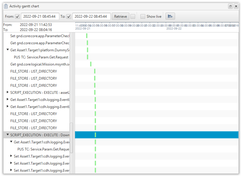
| The full details of each activity are displayed when you hover over the corresponding tree view entry. |
| Colour | Activity Status |
|---|---|
Light green |
Completed |
Aquamarine |
In progress |
Light sky blue |
Suspended |
Beige |
Idle |
Orange |
Aborted |
Red |
Failed |
Dark grey |
Timed out |
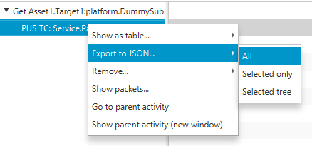
A context menu attached to the treeview items, shown in Figure 46, offers roughly the same options as the one in the activity log view. The only difference is the existence of the Export to JSON… option instead of Export to CSV…. If you save a file using this option, it can later be loaded into the Activity Gantt chart view, using the rightmost button on the view’s toolbar.
5. Transfers
The MCS supports both file transfers and bulk parameter transfers, this chapter explains how to administer large data transfers made to and from the spacecraft using these capabilities.
File transfers work via CCSDS CFDP, but whether this is supported or not will depend on your deployment. CFDP transfers can be both unacknowledged and acknowledged. Unacknowledged means that there is no guarantee of completeness – when errors are detected, data is discarded. This is fine when two-way communication is impossible, it’s fine to have incomplete data, or there are already other failsafes to ensure a successful transfer. Acknowledged provides error recovery through re-attempting the missing parts, but may not be possible if there is no two-way communication possible.
A bulk parameter transfer is a way to get data from a large parameter or one that has many rows. The works via ECSS PUS LDT protocol, whether this is supported or not will depend on your deployment. Parameter transfers can also use the Parameter Transfer Protocol defined by the MCS.
5.1. Downlinks
Parameter downlinks can be initiated by using the parameter view and clicking the downlink button, highlighted in Figure 47. This will initiate an LDT downlink (if supported by the OBSW), saving the file to the chosen destination.

This will initiate an LDT downlink (if supported by the OBSW), saving the file to the chosen destination. The right-hand side section of the download button allows the user to specify whether to downlink the parameter to a single or multiple files and via which protocol.
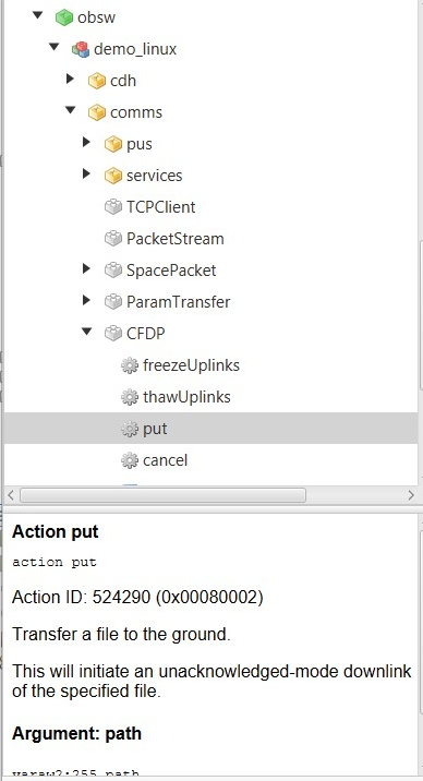
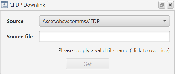
File downlinks can be initiated if the OBSW has the CFDP component. Within the CFDP component is an action for requesting the downlink of a file, shown in Figure 48. CFDP downlinks can also be initiated via the CFDP Downlink window available via the toolbar button highlighted in Figure 49.

This will bring up the CFDP downlink window, where you can specify a source file to downlink, as in Figure 50.
5.2. Uplinks
Parameter uplinks can be made in the same way as downlinks, both through the parameter view button highlighted in Figure 51, and through the CFDP. Clicking the uplink button will initiate an LDT uplink that uploads the contents of the parameter.

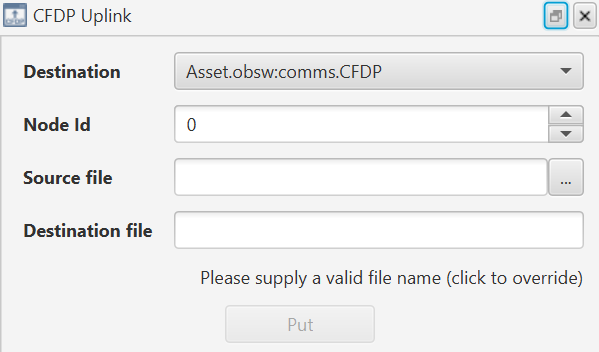
File uplinks are also available if the OBSW supports CFDP. You can use the CFDP Uplink window available on the toolbar to uplink files using CFDP, shown in Figure 52. This will bring up the CFDP uplink view, where you can specify a source file and a destination, as in Figure 53.

5.3. Viewing transfers
Transfers can be viewed from the transfers window, available from the toolbar through the button highlighted in Figure 54.

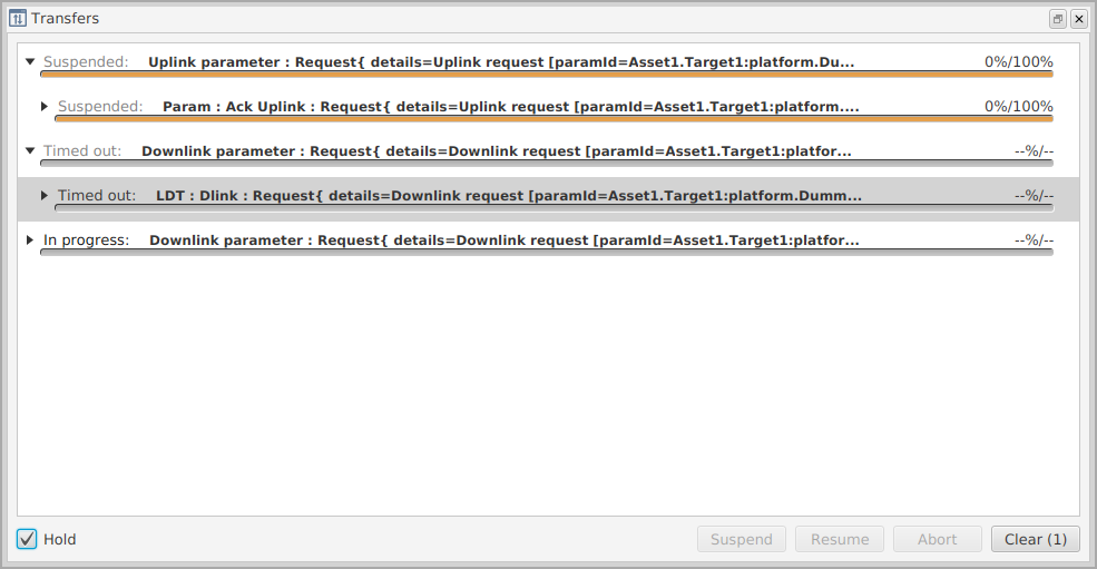
The transfers window displays active transfers. This window allows you to abort, resume and suspend active transfers. The hold checkbox will hold transfers that have completed whilst the checkbox is checked. Figure 55 shows what this will look like for transfers suspended, timed out, and in progress.
6. Internal scripting
Scripting is fundamental for automation within the MCS. The MCS supports a rich scripting environment that allows you to write isolated programs externally and run them within the MCS. Scripts are written in the Groovy language and allow direct access to an API allowing you to do various operations that the MCS can do itself, for example: getting and setting parameters, invoking actions, and initiating transfers.
| Groovy is a scripting language closely based on Java. Making use of the concepts in this chapter requires some knowledge of programming languages on the part of the user. |
Everything described in this chapter is internal to the MCS. There are additional methods of scripting via external programs based on gRPC and python, as described in Section 7.
6.1. Script executor
Scripts are typically run at pre-determined times as part of a ground schedule (see Section 8). However, a Groovy script can also be run immediately using the Script executor, accessed via the menu through "Monitoring" > "Script Execution…" or the toolbar button highlighted in Figure 56.

The script executor window can be seen in Figure 57. The ellipsis button, …, allows you to navigate through your computer and select the relevant Groovy script. Once this has been selected, the Execute button will become active. Clicking this button immediately executes the script.
| Multiple instances of the script executor can be created at the same time. They and the scripts selected in them can be saved as part of a layout, for quick execution during operation. |

6.2. Scripts
Scripts are executed by the MCS and provide access to core MCS functionality. The MCS provides built-in functions to allow you to issue commands to the MCS and indirectly to the spacecraft. For example, the example given in the previous section called the function getParsed with a string argument, getParsed is a function provided by the MCS. These functions allow you to interact with the MCS and therefore the OBSW. You can of course create your own methods as per the Groovy language specification depending on the complexity and usage of the script.
With larger scripts it’s recommended that you start splitting the functionality into classes and import these classes into the script, keeping the amount of code inside the script to a minimum. Any class available inside the scripts directory – including subdirectories – is available to import using the same conventions as normal Java or Groovy code.
The following sections will explain the various methods available to you whilst scripting in the MCS. HTML documentation for the full scripting API is included in the MCS installation directory, under /build/GNDSW/Groovy/scripting-api-docs.
6.2.1. Accessing core services
The getServices function returns a ServiceAssetSource object, which provides scripting access to many core MCS services. HTML documentation for this class, and for the services returned by its functions, is in the MCS installation directory, under /build/GNDSW/Groovy/services.
| The service classes and functions must be used with care, as they provide access to core MCS functionality. |
6.2.2. Logging
The scripting API gives you access to the system log. To access it, call the getLogger function. You can use this to append to the system log; this is a useful way of getting information out of your script and visible whilst it’s executing. The example below shows how to log an error:
getLogger().error("Now this is an error!")Verify the output in the server console.
6.2.3. Invoking actions
Invoking actions are executed using the i function. An i followed by the parameter name or ID will invoke the specified action. For example the code to invoke the Version.dumpVersion action would be:
i 'Asset.obsw.demo_linux:Version.dumpVersion'If successful the version should be dumped to the debug log in the connected deployment.
Some actions will need arguments passed to them. These can be passed to the i function as the second and subsequent arguments, following the action identifier. To invoke action core.Storage.wipe (which has a signature with a raw2 argument) using the decimal 1 as the argument, use the following command:
i 'Asset.obsw.demo_linux:core.Storage.wipe', [0x00, 0x01]The square brackets represent a list in Groovy. To send a list of bytes, separate each byte within the brackets with a comma. Decimal and binary values can also be used. Please refer to the Groovy language documentation for more information.
6.2.4. Getting parameters
You can get a parameter using the getParsed function.
getParsed 'Asset.obsw.demo_linux:platform.DummySubsys1.dummyParam32'The parsing converts the raw output, which will be represented as a Groovy object, to a readable string. This parsed form is useful if you need to print the value of a parameter to the screen but not so much use if you need to do further processing with it inside a script. To get the raw value use the g function:
g 'Asset.obsw.demo_linux:platform.DummySubsys1.dummyParam32'This will request the value from the OBSW and print the output to screen. It won’t be human-readable because it will output the raw representation of the parameter; in this case it will be an ArrayList. However, the benefit is that we can use this and derive the value from it in our own way.
For example, we can convert it to its string form by calling toString on the returned value:
g('Asset.obsw.demo_linux:platform.DummySubsys1.dummyParam32').toString()Which will return the string representation of the array.
For multi-row parameters you can use the g function with the first row, last row and resize arguments:
	g 'Asset.obsw.demo_linux:platform.DummySubsys1.multiRowParam',
		0, 10, true
This will perform a get for rows 0 to 10, resizing the result to fit the value. All parameters beyond the name argument are optional. In the case of multi-row parameters, eliding the resize flag will default to false, and eliding the last row will mean the remaining integer argument represents the index of a single row to get. The same arguments can be passed to the getParsed method to return a human-readable result.
6.2.5. Setting parameters
Setting parameters can be achieved by using the s function:
s 'Asset.obsw.demo_linux:platform.DummySubsys1.dummyParam32', 50Verify the value is set by getting the value:
getParsed 'Asset.obsw.demo_linux:platform.DummySubsys1.dummyParam32'This should now return 50.
As with the g method there are functions for setting multi-row parameters. To set a multi-row parameter use the multi-row s function:
	s 'Asset.obsw.demo_linux:platform.DummySubsys1.dummyParam32',
		0, [60,53,12,7,32], true
If dummyParam32 was a multi-row parameter, then this would set row 0 to the value 60, row 1 to the value of 53, row 2 to the value of 12, and so forth. The second argument is the first row to replace. The third argument is a list containing the values to set, the length of which determines the number of rows to replace. The fourth argument is the resize flag, here set to true, which means that the number of rows this parameter has would be resized to fit the number of elements in the list if needed.
6.2.6. Querying parameters
To query parameters for their metadata use the q function:
q 'Asset.obsw.demo_linux:Version.version'This returns a QueryResponse object. The QueryResponse contains all the fields of the standard OBSW query response. You can interrogate this object to expose various bits of metadata relating to the parameter. The available methods are:
   - getCurrentRowBytes
   - getCurrentRows
For example:
def metaData = q 'Asset2.Target2.deployment:Version.version'
getLogger().info("RowBytes = " + metaData.getCurrentRowBytes().toString())
getLogger().info("Rows = " + metaData.getCurrentRows().toString())
6.2.7. Transfer with scripts
Transferring data with scripts is a matter of calling the relevant methods: downlink and uplink. To downlink a parameter’s value, use the downlink function:
	downlink 'Asset.obsw.demo_linux:
		platform.DummySubsys1.dummyParam32', 0, 0, 1
This will downlink from row 0 to row 0; a single row downlink with the expected number of bytes per row set to 1. This will return a list of byte arrays, each representing a row.
For an asynchronous downlink of a parameter use:
	downlinkAsync 'Asset.obsw.demo_linux:Version.version', 0, 0, 4, {
		response, activity ->
			activity.getSuccessResult().ifPresent(result -> {
				getLogger().info(result.toString())
				getLogger().info("Data = " + result.getRowData())
			})
			activity.getFailureResult().ifPresent(result -> {
				getLogger().info(result.toString())
			})}
This example provides a callback with the activity and response, and will not block. Once completed, the callback provided as the last argument will be called. Within the callback access you can access a successful result via:
activity.getSuccessResult()This returns an Optional which wraps a GetResponse if the activity was successful.
The retrieved data (a byte array) is available via the result’s getRowData() function, as shown.
You can access a failure result by calling:
activity.getFailureResult()This returns an Optional which wraps an ErrorResponse if the activity failed.
To uplink to a parameter use the uplink function:
	uplink 'Asset.obsw.demo_linux:platform.DummySubsys1.dummyParam32',
		rows, 0, true
The rows argument is a list of byte arrays, each element in the list is a row. How you construct this list of byte arrays is up to you. You could for example create the list from a file on the file system and apply additional mutations to the sent data prior to uplink.
Transferring parameter blocks
Downlinking can be applied to parameters, as above, and parameter blocks. Parameter blocks are downlinked in a similar way, but you must use the downlinkBlock and downlinkBlockAsync methods instead, providing a block index as part of the arguments.
For a synchronous, blocking downlink of a parameter block for block index 1 with first and last row lengths both set to 0 and a byte row size of 4:
	downlinkBlock 'Asset.obsw.demo_linux:core.Storage.channelContent',
	 	1, 0, 0, 4
For an asynchronous downlink of a parameter block with a callback:
	downlinkBlockAsync 'Asset.obsw.demo_linux:core.Storage.channelContent',
		1, 0, 0, 4, {response, activity ->
		getLogger().info(activity.getResponse().toString())}
6.2.8. Listening to state changes in downlinks
It might be the case that you need to respond to when a transfer moves from in-progress to suspended. To do this, provide a state listener callback as the final argument to the downlinkAsync or downlinkBlockAsync functions:
	downlinkAsync 'Asset.obsw.demo_linux:core.Storage.numRows', 0, 5, 256,
		{r,c -> }, {transfer -> getLogger().info(transfer.
		getState().toString())}
This will supply the transfer to the callback whenever the transfer changes state, and log its state to the log view. The available states can be used by importing:
com.brightascension.coast.activity.ActivityStateThe available states are:
-
IDLE
-
IN_PROGRESS
-
COMPLETED
-
FAILED
-
SUSPENDED
-
ABORTED
-
TIMEOUT
6.2.9. Executing scripts inside scripts
If you want to trigger the execution of another script inside a script that’s currently running, you can use the following method:
executeScript 'example.groovy'This will execute the script example.groovy inside an existing script, halting progress of the current script until the child script completes execution. The script name passed to this method is relative to the MCS Server’s root directory. To execute scripts external to this directory, you can pass a File instance representing the location of your script, or simply specify the absolute path of the script:
executeScript 'C:/scripts/example.groovy'6.2.10. Updating onboard schedules
Schedules can be administered by the Groovy Scripting API via onboard Action components. To access this interface call one of the following functions inside a script. (The string argument is the fully qualified component identifier for the script target):
	eventActionComponent 'Asset.obsw.demo_linux:cdh.EventAction'
	timeActionComponent 'Asset.obsw.demo_linux:TimeAction'
	periodicActionComponent 'Asset.obsw.demo_linux:PeriodicAction'
These functions return an object that represents the equivalent onboard component. Each of these returned objects allows you to uplink a schedule via:
uplinkSchedule(entries, resultCallback)The entries argument is a list of internal MCS classes that represent each schedule entry to uplink. You can create a list of these entries from a CSV file that’s been exported by one of the corresponding onboard schedule GUIs inside the MCS, as shown in the following example for uploading a Time Action Schedule.
First, load the schedule entries from the CSV file:
import com.brightascension.coast.model.activity.ActivityState;
import com.brightascension.coast.model.ComponentIdentifier;
import com.brightascension.coast.lib.component.auto.ScheduleComponent.UplinkScheduleNotifier;

def componentName = "Asset1.Target1.Deployment:cdh.TimeAction"
def file = new File("scripts/timeActionSchedule.csv")
def taComponent = timeActionComponent(componentName)

List<TimeActionScheduleEntry> entries = getServices().getScheduleManagementService().convertTimeActionScheduleFromCsv(ComponentIdentifier.fromString(componentName), file.bytes)

List<byte[]> encodedEntries = getServices().getScheduleManagementService().encodeTimeActionSchedule(ComponentIdentifier.fromString(componentName), entries)

getLogger().info("Encode and uplink flight plan for: Asset with file: " + fileName)
Then uplink these entries to the spacecraft:
// First, clear the schedule component
i taComponent + '.clear'

taComponent.uplinkSchedule(entries, new UplinkScheduleNotifier() {
    @Override
    public void onScheduleUplinkFinished(ActivityState state, String failureDescription) {
        if (failureDescription == null || failureDescription.isEmpty()) {
            getLogger().info("Encode and uplink flight plan completed from file: " + fileName)
        } else {
            getLogger().error("Encode and uplink flight plan failed: " + failureDescription)
        }
    }

    @Override
    public void onError(Optional<Exception> e) {
        getLogger().error("Error uplinking flight plan: " + e.map(ex -> ex.getMessage()));
    }
})
7. External scripting
7.1. Python API
The Python API is provided alongside the MCS as a means of scripting via an external program, and communicates with the MCS via gRPC. The mcs_client Python API is built on top of the asynchronous programming library asyncio, for more details on this see the library’s documentation (https://docs.python.org/3/library/asyncio.html) as well as the documentation and examples provided with the mcs_client Python API itself.
The Python API can be used as a means of automation, by creating and executing an external Python API script of MCS commands. It supports complex stacks and high-level tasks, with debuggers allowing manual control of the script that is not possible via other methods of automation, such as ground schedules or procedure execution.
Additionally, the Python API provides access to most useful Services and Service Operations provided by the MCS, and exposes these as methods on the Python API Service Client. Operations of the Python API Service Client are intended to be coarse grained and represent the parent activity of, for example, a file transfer within an MCS. The operations should either complete successfully, or fail with an appropriate exception. These top level activities can be monitored for progress, suspended, and resumed as in the MCS. However, the Python API doesn’t actively expose the sub-activities of the top level activities, for example, file transfers. If you wish to examine in more detail the reason for a failure by looking at the sub-activities of an operation the recommendation would be to use the Activity Gantt Chart available in the MCS GUI.
Full documentation of the Python API is available at: GNDSW/python/mcs_client/docs/html/index.html.
7.1.1. Capabilities
The Python API allows a user to make use of a Service Client to perform a range of tasks in the MCS. It can access most MCS services, including procedure execution. Examples of tasks that can be completed via the Python API include:
-
Get and Set the values of onboard parameters
-
Query the dimensions of an onboard parameter
-
Invoke onboard actions
-
Uplink and Downlink large parameters over multiple transfer frames
-
Register to receive onboard Event, Housekeeping and Debug telemetry
-
Initiate transfers
-
Decode aggregations (e.g HK beacons)
This interface also allows a user to explore the spacecraft database to:
-
Lookup onboard identifiers
-
Fetch descriptions of onboard components, events, actions parameters, etc.
A table listing all services and operations available via the Python API is below:
| Service | Operations |
|---|---|
Action |
invoke, arm_critical, invoke_critical, disarm_critical |
Activity |
get_activity_state_by_type, suspend_activity, resume_activity, abort_activity, get_activity_status, monitor_activity |
Aggregation |
add_aggregation_from_file, add_aggregation, remove_aggregation, get_aggregation_definition, encode_aggregation_definition, decode_aggregation_definition, decode_aggregation, decode_aggregation_from_filepath, get_aggregations |
Archive |
ingest_aggregation, ingest_aggregation_from_filepath, ingest_event_log, ingest_event_log_from_filepath |
Beacon |
add_beacon_mapping, remove_beacon_mapping, monitor_beacons, get_beacon_mappings, remove_aggregation_beacon_mappings |
Connection |
add_connection_point, set_connection_point, add_child_connection_point, remove_connection_point, get_connection_point_configuration, get_connection_point_summary, get_connection_points_summary, get_asset_connection_points_summary, open_connection, mark_connection_for_sending, close_connection, close_connections_for_asset, close_all_connections, copy_connection_point, move_connection_point |
Event |
monitor_events, decode_event_log_from_filepath, decode_event_log |
File transfer |
uplink_file, downlink_file |
Mission |
add_asset, remove_asset, add_target, get_asset_properties, set_asset_properties, get_target_properties, set_target_properties, remove_target, add_deployment, remove_deployment, set_current_deployment, get_current_deployment, get_deployment, get_assets, get_targets, get_deployments_for_asset, get_deployments_for_target, get_deployment_details |
Parameter |
get_max_size_get, get_max_size_set, set_max_size_get, set_max_size_set, get, set, query, monitor_parameters |
Procedure execution |
execute, get_procedure_definition_identifiers, get_procedure_instance_identifiers, get_procedure_instance_identifiers_by_procedure_def_name_version, get_procedure_instance, get_procedure_instances, get_procedure_definition, get_procedure_definition_xml, convert_procedure_definition_xml, convert_procedure_definition, add_procedure_instance, import_procedure_definition, add_procedure_definition, rename_procedure_definition, rename_procedure_instance, remove_procedure_instances, delete_procedure_definition |
Schedule |
encode_time_action_schedule, decode_time_action_schedule, time_action_schedule_from_csv, time_action_schedule_to_csv, time_action_schedule_from_yaml, time_action_schedule_to_yaml, encode_event_action_schedule, decode_event_action_schedule, event_action_schedule_from_csv, event_action_schedule_to_csv, event_action_schedule_from_yaml, event_action_schedule_to_yaml, encode_periodic_action_schedule, decode_periodic_action_schedule, periodic_action_schedule_from_csv, periodic_action_schedule_to_csv, periodic_action_schedule_from_yaml, periodic_action_schedule_to_yaml, encode_lean_time_action_schedule, decode_lean_time_action_schedule, lean_time_action_schedule_from_csv, lean_time_action_schedule_to_csv, lean_time_action_schedule_from_yaml, lean_time_action_schedule_to_yaml, encode_schedule_from_csv, encode_schedule_from_yaml, decode_schedule, decode_schedule_to_csv, decode_schedule_to_yaml, encode_auto_schedule, decode_auto_schedule, decode_auto_schedule_results, auto_schedule_from_yaml, auto_schedule_to_yaml_bytes, auto_schedule_results_to_yaml_bytes |
Transfer |
uplink, downlink, downlink_to_file, uplink_from_file |
7.1.2. How to run
Access to the Python API MCS client and Procedure Execution client are provided in the MCS client-server distribution as part of a release.
Installation information for the Python API can be found within the 'README' file in the 'GNDSW/python/mcs_client' folder within the release.
7.1.3. Accessing services
All MCS and Procedure Execution service Python classes are provided in 'GNDSW/python/mcs_client/dist/mcs_client-22.2/mcs_client/service', and similar for procedure execution. Here, all of the interface classes can be viewed, so in each service class each we can see every supported method and what arguments they require. Examples of each service being called in a separate Python script can be found in 'GNDSW/python/mcs_client/examples'.
8. The Ground Schedule
The ground schedule in the MCS is a scheduling system that allows absolute- and relatively-timed jobs to occur, allowing you to plan schedules based around certain events. The ground schedule can be accessed from the menu via Monitor → Time based schedule, not to be confused with the on-board schedule builders found under the Tools section of the menu and covered in Section 9. It can also be accessed from the toolbar via the button highlighted in Figure 58.

Upon start up the ground schedule will automatically reactivate and upon shutdown the ground schedule will deactivate. Jobs scheduled for periods when the MCS is not currently running will never be executed.
The ground schedule is managed by the Time schedule view as shown in Figure 59. Ground schedule entries can have an absolute timestamp, or they can be timed relatively to another entry, with an offset specified in seconds. With this in mind a relative schedule entry can be relative to another relative schedule entry, all the way back to a ‘root’ absolute entry. Offsets can be set to negative or positive – negative offsets mean the relative entry will trigger before the trigger of its parent.
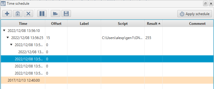
Clicking the plus button will add an absolute schedule entry with the time set to the current MCS time. Selecting the new entry and clicking the smaller plus button will add a relative entry. The offset can be edited by clicking on the offset cell for the newly created entry. The computed time to execute the relative entry is updated when you update the offset.
Updating the timestamp of an absolute entry will update all timestamps for the other entries underneath or relative to it.
Edits to the ground schedule are only applied and saved once you click and confirm the Apply schedule button at the top right of the view.
The pause button will temporarily prevent any scheduled entries from being executed. Un-toggling the button will resume execution.
Entries can be removed using the delete button on the toolbar, or by pressing the delete key with entries selected.
8.1. The ground schedule entry
The ground schedule entry is composed of several fields:
-
Scheduled time (this is computed for relative entries)
-
Offset in seconds (this does not exist on absolute entries)
-
Label – a free-form text value that will be shown when referring to this schedule entry in logs
-
Script – the path to a script to execute when this schedule entry is triggered. This is optional, an entry without a script may be used as an anchor point for further relative entries
-
Result – once the entry has been triggered the last statement of the script to execute will be dumped to this value, this value is read only
-
Comment – a free-form text value that will be shown only when viewing the Time schedule GUI
To edit the label, comment or script of an entry, simply click the relevant row and column. You can try pointing an entry to the example.groovy script and scheduling it to occur in the future. (Remember to click the Apply schedule button to apply your changes.) The example.groovy script will send various log messages to the system log. You can verify it executes successfully by keeping an eye on the MCS Server console.
8.2. Importing and exporting
You can import and export ground schedules from the MCS. To export a ground schedule simply click the save button. To import another ground schedule click the open button. Remember to click the Apply schedule button to apply an imported schedule.
8.3. Colour indicators
Schedule entries are coloured depending on their state. The colours indicate success, warning and error states. Below is a table indicating the colours and their respective states:
| Colour | Schedule entry state |
|---|---|
Green |
A script successfully executed |
Amber |
A script did not execute, although its schedule time has passed |
Red |
A script tried to execute but failed |
White |
A script is scheduled to be executed in the future |
A success indication means that the schedule entry executed and returned with a non-negative number or a non-number.
An amber warning indication occurs when a schedule entry never executed – this could be due to it already being in the past when it was created or if the MCS was not active to service the entry due to it being shutdown or paused when the scheduled entry was supposed to occur.
An error indication is triggered when the script fails either on the MCS – either through a compilation or connection error, or on the flight-side when the script attempts to interact with the spacecraft and fails. If a script returns with a negative numerical value then this will also trigger a failure, to indicate that your intentions within the script failed.
8.4. External ground schedule polling
A mechanism in the MCS exists to poll the filesystem for external ground schedule entries to be imported into a running instance of the MCS. This allows you to place a ground schedule in the exported portable JSON format in a configurable watch directory which the MCS will then poll. The configuration settings are described in Section 11.1.5.
A groundScheduleIngesterPollingDelay number greater than 0 indicates that external ground schedule polling should be enabled and the polling mechanism will occur based on this delay in seconds.
How the MCS treats ingested schedules depends on the name of the file. If the file is appended with add.json the entries stored in this JSON file will be added to the existing ground schedule. If the file is appended with new.json the entries stored in this JSON file will replace the entire ground schedule at once.
Once the MCS ingests a ground schedule it will either digest or reject the JSON file. If it successfully reads the schedule it will move the ingested file into the digested directory relative to the polled directory. If it fails to import for one reason or another an error will be printed to the MCS system log and the file will be moved to the rejected directory, again relative to the polled directory.
9. On-Board Schedules
The on-board schedule functions provided by the OBSW are components which are displayed in the mission explorer’s asset tab alongside the other components in the loaded deployment. A schedule consists of one or more entries, each with an execution time value, an on-board parameter or action identifier, and any argument values to be provided to the parameter or action. The on-board schedule components encode schedules as packed entry parameters, and the on-board schedule builder views allow you to view and edit schedules in a more readable form. These can be accessed via the Tools menu (Figure 60).
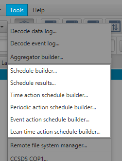
The views for schedules in the TimeAction, PeriodicAction and EventAction components can also be accessed by right-clicking the relevant component in the mission explorer and selecting Administer.
|
The following schedule components are supported by the on-board schedule views:
-
Schedule (Section 9.1)
-
TimeAction (Section 9.2)
-
PeriodicAction (Section 9.3)
-
EventAction (Section 9.4)
9.1. Schedule Component
To execute an on-board schedule using the schedule component, use the schedule builder view to build the schedule and save it as a binary file, which can be uploaded to the flight-side Storage component. After execution, you can download results from the ScheduleResultsLogger component, and view the results in the schedule results view. These steps are described in detail in the following subsections.
9.1.1. Schedule builder
The schedule builder view (Figure 61) allows you to create, view and edit on-board time-based schedules for deployments containing the schedule component. The schedule component is intended to replace the legacy TimeAction component.
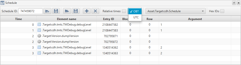
After selecting the schedule component in the relevant asset and target from the toolbar dropdown, you can create a new schedule by adding entries using the + button, or open an existing saved schedule - either in the YAML format saved by the MCS, or in the binary format which is uploaded to the spacecraft.
| If you are creating a new schedule based on an existing one loaded from a file, you are recommended to enter a new random value in the schedule ID field in the builder view, so that the old and new schedules, and their respective results, can be distinguished by the on-board and MCS software. |
The timestamps for a schedule can be defined as relative or absolute values. This is a single setting for each schedule: it cannot contain a mixture of entries with relative timestamps and entries with absolute timestamps. If absolute values are chosen, they can be displayed as numerical On-Board Timestamp (OBT) values, or converted to UTC date and time using the time correlation settings for the selected asset and target (see Section 15).
Relative time values represent the number of elapsed seconds to wait before executing a step. The first step is executed when its relative time value has expired after the schedule is activated by setting the schedule component’s channelId parameter to the Storage channel containing the schedule.
Each new schedule and entry is given a unique identifier, which is required by the schedule component. These identifiers are displayed in decimal or hexadecimal format, controlled by the checkbox in the builder window’s toolbar.
Entries can be moved relative to one another using drag and drop. They can also be moved or duplicated using the ctrl-C / ctrl-X / ctrl-V clipboard shortcuts for copy / cut / paste.
|
You can save a schedule to the portable YAML format by clicking the first Save button. The textual YAML file can be edited manually, or reloaded into the schedule builder view.
9.1.2. Uploading Schedules
Use the second Save button in the schedule builder view to encode and save the schedule in the binary format required by the on-board schedule component. The MCS will not allow a schedule to be encoded if any of the entry timestamps are in descending order, as this would lead to the schedule being rejected by the on-board schedule component.
When connected to the target system, you can upload an encoded schedule by accessing the channelContent element in the target’s Storage component, and clicking the uplink from file button (outlined in red in Figure 62).
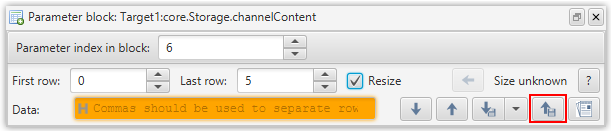
Enter the channel number in Parameter index in block, to select the Storage channel where the schedule should be stored. This must be greater than zero, and the channel row length should be 19, as shown in the Storage.rowLength value for the channel index.
If a schedule has already been activated, the schedule component’s channelId value will indicate the Storage channel where the current schedule is stored, and the channel will be claimed, blocking uploads. (This is reflected in the Storage.isClaimed value for the channel index.) In this case, if you intend to upload a new schedule to the same channel, you must change the schedule component’s channelId (for example, to zero), before executing the upload.
|
The binary file length (in bytes) should be an exact multiple of 19. Where the number of 19-byte rows contained in the file is n, you must set the First row and Last row values to 0 and (n-1) respectively. Select the Resize checkbox to ensure that the number of bytes stored in the channel will be no more or less than the contents of the file after the upload.
After uploading the file, set the schedule component’s channelId value to the Storage channel containing the uploaded schedule. The schedule steps should now be executed according to their respective Time values.
To record schedule execution results, set the ScheduleResultsLogger component’s channelId parameter to an available Storage channel. This must be greater than 0, and not equal to the schedule component’s channelId, or any other channel which is already claimed by another component.
|
9.1.3. Downloading Results
Schedule execution results stored by the ScheduleResultsLogger component can be downloaded to a binary file from the Storage component, via the channelContent parameter. Set the Parameter index in block to the ScheduleResultsLogger’s channelId value, hit the question-mark button to find the number of rows stored, and the left-arrow button to populate the First row and Last row values, before clicking the Download to a file button. The binary results file can then be viewed in the schedule results view (Figure 63), which is accessed through the Tools → Schedule results menu option.
After downloading the schedule results, you can clear the results log channel using the Storage component’s wipe action, specifying the channel where the results are stored, so that the same results will not be included in future downloads. You need to set the ScheduleResultsLogger’s channelId parameter temporarily to another value (typically, zero) to release the claim on the channel before invoking the wipe action.
|
9.1.4. Schedule results view
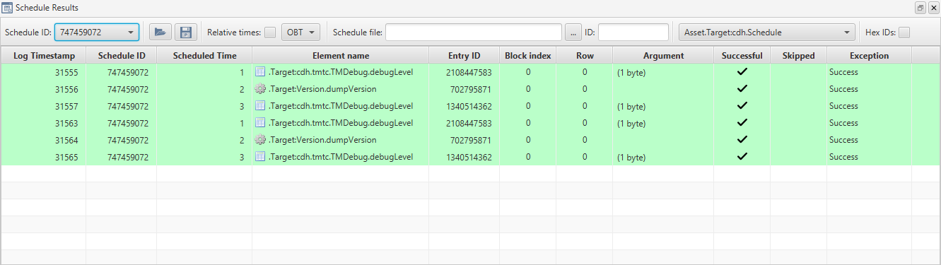
A schedule results file can include the results of multiple runs of a schedule, and the results of multiple schedules. In the latter case, you can select to view results from a single schedule using the dropdown at the left of the toolbar. As can be seen from the illustration, the viewer is similar to the schedule builder view, except that it is a read-only view, and it includes log timestamp and schedule ID columns. Each table row is coloured according to the corresponding entry status: green for success, red for failure.
The results files include parameter sizes instead of values. Values can be displayed by loading a schedule YAML (Figure 64) for a schedule with a unique identifier matching one in the results file.
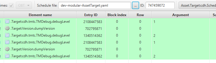
When displaying the results of a schedule whose YAML file has been loaded, additional row colours are used to indicate unmatched schedule entries or unmatched results. These row colours are described in Schedule results view row colours.
Displayed results from a single selected schedule can be saved in YAML format for external processing or analysis. The MCS does not include the capability to load such YAML results files.
| Colour | Meaning |
|---|---|
Green |
A success entry in the results file with a matching entry in the schedule file. |
Red |
A failure entry in the results file with a matching entry in the schedule file. |
Amber |
An entry in the results file with no matching entry in the schedule file. |
White |
An entry in the schedule file with no matching entry in the results file. |
9.2. Time action schedule builder
The Time Action schedule Builder (Figure 65) allows schedules dependent on time to be constructed and can be opened by going to Tools → Time action schedule builder.

Schedule entries (rows in the table) uploaded to the target can be executed at an absolute time; the onboard time (OBT) at which the entry will be executed. Absolute time entries can also be provided in date-time format if time correlation is supported. The time format displayed in the table can be changed using the dropdown in the toolbar (Figure 66).

While OBT is selected, the user will only be able to manually add absolute-time values into the table in OBT, and vice versa for UTC. When importing a CSV, YAML or encoded schedule file via the load button, the entries can be specified in OBT or UTC time, but they will be displayed in whichever time format is selected in the dropdown at the time. Alternatively, the entry can be run at a relative time; the time at which the entry will be executed is given as an offset to the OBT. Switching the display between OBT and UTC format will not affect relative entries. Once a schedule entry’s relative or absolute time is reached, a parameter or action associated with the entry can be set or invoked, respectively. The schedule can later be downlinked to check whether it has been executed.
9.3. Periodic action schedule builder
The Periodic Action schedule Builder (Figure 67) allows the construction of schedules that run at regular intervals and can be opened by going to Tools → Periodic action schedule builder. Once uploaded, an entry in the schedule is executed every Period seconds, and are run a total of Multiplier times, each time either invoking an action or setting a parameter. The schedule can later be downlinked to check whether it was executed.

9.4. Event action schedule builder
The Event Action schedule Builder (Figure 68) allows the construction of schedules that run according to whether certain events occur, and can be opened by going to Tools → Event action schedule builder. Each entry in the schedule contains an event that, when it occurs, causes an action to be invoked or parameter set. The schedule can later be downlinked to see whether it was executed.

9.5. Uplinking and downlinking TimeAction, PeriodicAction and EventAction schedules
These components store schedules themselves, instead of using the Storage component. The uplink and downlink buttons found on the toolbar allow you to transfer a schedule to and from the respective component.
| If you uplink a schedule with no entries, it is assumed you want to clear the schedule – this will invoke the OBSW component’s clear action, removing all entries. |
9.6. Schedule entries
Onboard schedule entries vary between components but they will all possess several fields in common:
-
Action or parameter indicator – this is either a cog icon for actions or a note icon for parameters
-
Element name — this is the action or parameter name to invoke or set
-
Parameter row — the parameter row of this schedule entry, only applies to a parameter
-
Enabled flag – this indicates whether or not the entry can be triggered
-
Executed flag – a read only flag to indicate whether or not the entry was executed
-
Argument – the argument passed to either the parameter being set or the action being invoked
All these fields are visible on the view as columns in the table of schedule entries. Other columns will also be visible but will vary depending on which on-board component you are viewing, for example event action will include the event ID and time action will include the time in milliseconds.
You can add schedule entries by clicking the + button and remove schedule entries by clicking the x button with entries selected.
9.7. Colour indicators
Downloaded schedule entries are highlighted depending on state. Green indicates success, red failure. A highlighted red border when uplinking indicates there’s a problem with this particular schedule entry and you’ll need to remedy the issue by looking at the system logs and changing the relevant field values.
The green success state correlates to the executed flag being true. The red failure state only occurs in certain circumstances, for example on the TimeAction component this will trigger if the schedule entry is expired but not executed indicating a possible failure.
9.8. Importing and exporting
On-board schedules can be exported to CSV or YAML by clicking the save button, and administered outside the MCS. They can likewise be imported using the open button, and uplinked or edited in place (Figure 69).

On-board schedules can also be exported and imported in the binary encoded format used in the on-board component, using the other open and save buttons (Figure 70).

10. Calibrations and checks
This chapter explains how to set up calibration functions and validation checks for parameters. Calibration functions are applied to parameter values to transform a raw value to a calibrated value. Checks can be applied to both raw and calibrated parameter values, and allow you to configure warning and error indicators for parameter values which are outside the norm.
Three files, in addition to the spacecraft SCDB file, are used to detail the relevant calibrations and checks. These files must be supplied when a deployment is added/updated
either via the Manage Mission display when using a GUI or
via the mission management service when using the Python API.
For the three files, one defines the calibrations, one defines the checks, and the third is used to associate those defined calibrations and checks to specific parameters in a deployment. This separation allows calibrations and checks to be used for multiple parameters.
10.1. Calibrations
The calibration definition file holds the parameter calibration definitions in YAML format.
The name field is the calibration identifier, used in the parameter definitions file to reference the calibration. The other fields are calibration type dependent.
10.1.1. Linear calibration
Converts using a result = Mx + C formula
-
mfield contains the M factor to use -
cfield contains the C value to add -
precisionfield contains the number of decimal places to truncate to
- linear:
    name: linear-calibration-example
    m: 0.25
    c: 0.001
    precision: 2
Calibration id of linear-calibration-example, input value is multiplied by 0.25, and has 0.001 added to it before being truncated to 2 decimal places.
10.1.2. Range calibration
Maps an input value from a range to a single value:
-
rangesfield contains a list of ranges asfrom:to:evaluateTotriples
- range:
  name: range-calibration-example
  ranges:
    -
      from: 0
      to: 10
      evaluateTo: 10
    -
      from: 11
      to: 100
      evaluateTo: 11
Calibration id of range-calibration-example, from 0 to 10 return 10, from 11 to 100 return 11.
10.1.3. Textual calibration
Maps input value from numeric to textual value. Where ranges of numeric values have particular significance, this can be combined with a range calibration (see Chain calibration, below).
-
mapsfield contains a list of mappings asfrom:topairs. Any input value not represented in this list will be mapped to a null output.
- text:
    name: text-calibration-example
    maps:
      10: "ten"
      11: "eleven"
Calibration id of text-calibration-example, map from 10 to Ten, map from 11 to Eleven.
10.1.4. Time calibration
Maps input value from numeric to time value:
-
offsetfield contains the offset to add to the input numeric value to adjust it to the January 1st 1970 GMT epoch -
scalefield denotes whether the numeric value is in seconds or otherwise assumed to be milliseconds. It is assumed that the numeric value is offset from January 1st 1970 GMT
- time:
    name: time-calibration-example
    offset: 0
    scale: seconds
Calibration id of time-calibration-example, times are in seconds since 1/1/1970.
10.1.5. Chain calibration
Applies a chain of other calibrations to the input value:
-
calibrationsfield contains the ordered list of calibrations to apply
- chain:
    name: chain-calibration-example
    calibrations:
      - range-calibration-example
      - text-calibration-example
Calibration id of chain-calibration-example, apply calibration id range-calibration-example, then apply calibration id text-calibration-example to the output of the previous stage.
So if the value of 77 was received, the first calibration (Range) is applied and returns 11, then the second calibration (Text) is applied and returns Eleven.
10.1.6. Polynomial calibration
Applies a polynomial calibration to input value:
-
degreesfield contains a mapping of degree to multiplier -
precisionfield contains the number of decimal places to truncate to
- polynomial:
    name: polynomial-calibration-example
    degrees:
      0: -32
      1: 245
      2: 0.23
      3: -1.67
    precision: 2
Calibration id of polynomial-calibration-example produces:

— where the input value is x and the result of the calibration is y, before being truncated to 2 decimal places.
For more examples, see the example calibration definitions file in:
./configs/calibrationDefinitions.yaml10.2. Checks
Checks are applied to parameter values to indicate warnings or errors on parameter values.
The check definition file holds parameter check definitions in YAML format. As for calibration files, the name field is always the check identifier, used in the parameter definitions file to reference the check.
You must set the ground parameter core.app.ParameterCheck.enabled to 1 (enabled) for checks to be applied.
|
10.2.1. Range check
Checks input value is inside lower ≤ value ≤ upper a named range:
-
labelfield is the check label (used when chained together to know which check has violated) -
severityfield is the severity level, one ofERROR,WARNING, orINFO -
lowerfield is the lower range value -
upperfield is the upper range value
| Any range value can be omitted and the relevant max/min value for the value type will be used instead |
- range:
    name: test-range
    label: HARD
    severity: ERROR
    lower: 1
    upper: 10
Check id of test-range named HARD, with a level of ERROR and valid range from 1 to 10.
10.3. Associations
The parameter associations file holds the parameter to calibration/check associations, in YAML format.
The name field represents the full name of the parameter instance in the SCDB. The remaining fields link to definition ids found in the calibration and check definition files respectively.
---
- existing:
    name: "Target1:platform.DummySubsys1.dummyParam8"
    calibrationId: text-calibration-example
    rawCheckId: large-range
    calibratedCheckId: small-range

- existing:
    name: "Target1:platform.DummySubsys1.dummyParam16"
    calibrationId: linear-calibration-example
    rawCheckId: large-range
    calibratedCheckId: small-range-HARD

- existing:
    name: "Target1:cdh.DataPool.platform.DummySubsys1.dummyParam32"
    calibrationId: chain-calibration-example
    rawCheckId:
calibratedCheckId: large-range| If using the GUI, the Parameter Log view allows you to view the results of calibrations and checks on parameter values. See Section 4.3 for more details. |
11. Configuration
11.1. MCS Server
To configure the MCS Server, key-value properties can be specified in MCS_Server/configs/mcs.properties. This editable text file contains one property per line, in the format <key>=<value>. The comment lines at the start of the file are generated by the MCS Server at startup. An example of this file is shown below:
#Comment
#Fri Sep 09 14:13:35 BST 2022
archiveRetrieval_enabled=JPA
influxDbV1_enabled=true
csvLogging_enabled=false
influxDbV2_store_enabled=true
The properties that can be modified are given in tables below.
11.1.1. General
| Configuration id | Field type | Default value | Description |
|---|---|---|---|
activityPersistenceDaemonDelay |
Integer |
10000 |
The delay in milliseconds between the persistence of activities to disk |
activityPersistencePath |
String |
data/active_activities |
Path to the directory activities are stored. |
configurationStoreFilePath |
String |
data/mcsConfig.data |
Path to the file containing cached or imported Ground parameter values. |
groundSchedulePath |
Directory |
schedules |
Default directory to look for ground schedules |
maxLogFileRecords |
Integer |
30000 |
The maximum number of records permitted inside the log archive CSV file. Exceeding this value will result in the current log being rotated to a separate file and further logs appended to a new file. |
missionRepository |
String |
data/missionFilestore |
Directory in which the MCS stores data about the current mission, such as assets and targets. |
remoteAccessPort |
Integer |
50051 |
The TCP port to which MCS Display clients can connect. |
timezone |
String |
UTC |
Timezone for displayed date/time values. Format should be accepted by java.time.ZoneId.of(String). |
11.1.2. Uplink/Downlink transfer
| Configuration id | Field type | Default value | Description |
|---|---|---|---|
downlinkTempPath |
Directory |
data/ldt_ parts |
Directory to store partial downlinks |
transferFilestorePath |
Directory |
cfdp_ filestore |
Directory in which CFDP downlink data, of completed transfers, is stored. |
transferTempFilestorePath |
Directory |
data/cfdp_ parts |
Directory where in-progress CFDP transfers are stored. |
11.1.3. Archiving
| Configuration id | Field type | Default value | Description |
|---|---|---|---|
archivePath |
File |
data/missionArchive/ |
The path to the archive |
archiveRetrieval_enabled |
String |
influxDbV2 |
Which archive to use for retrievals, this value can be either 'JPA' or 'influxDbV2' |
minimum_activity_date |
String |
None |
An optional field which, if populated, will prune all archived activity data with a timestamp before the date specified in this field. For example, setting 'minimum_activity_date=2023-01-01' in mcs.properties will prune all activity data from before 2023-01-01 on startup of the MCS. Depending on how large a data set is, this action might take some time to complete. |
11.1.4. Influx
| Configuration id | Field type | Default value | Description |
|---|---|---|---|
influxDbV1_enabled |
Boolean |
false |
Whether to enable storage using the V1 implementation of the Influx database |
influxDbV1_url |
String |
The URL for the Influx database |
|
influxDbV1_dbName |
String |
BAL_MCS |
The name of the Influx database |
influxDbV1_uname |
String |
Username to use to connect to the Influx database |
|
influxDbV1_pword |
String |
Password to use to connect to the Influx database |
|
influxDbV1_storeParams AsAgnostic |
Boolean |
false |
Store parameters in the archive as |
influxDbV2_store_enabled |
Boolean |
false |
Whether to enable storage using the V2 implementation of the Influx database |
influxDbV2_url |
String |
The URL for the Influx database |
|
influxDbV2_orgId |
String |
The organisation ID to use to connect to the Influx database |
|
influxDbV2_token |
String |
The authentication token to use to connect to the Influx database |
|
influxDbV2_storeParams AsAgnostic |
Boolean |
false |
Store parameters in the archive as |
11.1.5. Scripting
| Configuration id | Field type | Default value | Description |
|---|---|---|---|
scriptRoot |
Directory |
Directory in which scripts are placed to run via MCS’s |
|
groundScheduleIngesterPollingDelay |
Integer |
0 |
Time in seconds to poll the watched ground schedule directory. 0 indicates it should never poll and effectively switches this functionality off. |
groundScheduleIngesterPollingDirectory |
String |
ground_schedule_watch |
The directory to watch for new ground schedules or entries, relative to the MCS installation directory |
11.1.6. Security
When using CCSDS Space Link security, a YAML file is used to configure the security associations. An example YAML configuration is provided in the configs folder.
Security association parameters gives the properties that can be configured.
| Property | Field type | Default value | Description |
|---|---|---|---|
securityParameterIndex |
Integer |
The SDLS security parameter index. |
|
vcid |
Integer |
The virtual channel to match on |
|
applyToTc |
Boolean |
Should be |
|
applyEncryption |
Boolean |
Should be |
|
applyAuthentication |
Boolean |
Should be true if authentication is used, otherwise |
|
authenticationKeyHexString |
String |
The authentication string in Hex. |
|
encryptionKeyHexString |
String |
The encryption key string in Hex. |
|
initialisationVector |
Integer |
Provided as input to some cryptographic algorithms before processing user data. This serves to preload the cryptographic process and enhance its security by adding variability. |
11.2. MCS Display
To configure the MCS Display, key-value properties can be specified in MCS_Display/configs/display.properties.
The MCS maintains numerous properties in this file which should not be modified.
The properties which can be modified are given in Display configuration parameters.
| Property | Field type | Default value | Description |
|---|---|---|---|
enableDeploymentIdCheck |
Boolean |
true |
Allows deployment checking to be disabled, meaning the flight-side will not reject commands if the deployment id on the flight and ground do not match. |
groundStations |
String |
List of ground stations to display on the map. Formatted as a triple of name of the station followed by the latitude and longitude in degrees. To specify multiple stations, simply list multiple triples separated by a colon. For example: |
|
mapLatParameters |
String |
Parameter representing spacecraft latitude. For example, |
|
mapLonParameters |
String |
Parameter representing spacecraft longitude. For example, |
|
mapTimestampOffsetMs |
Integer |
0 |
|
mapTrailLength |
Integer |
100 |
Maximum number of lat-lon points in the trail of a spacecraft trail displayed on the map. |
scriptPath |
Directory |
scripts |
Default directory to look for script files. |
12. Housekeeping
The Housekeeping tab in the mission explorer allows you to view and update the aggregations which are used by the on-board software to transmit housekeeping (system status) and other data. Aggregations are used by on-board Beacons to send regular updates, and the Housekeeping tab also allows you to map aggregations to Beacon IDs, to enable the decoding of Beacon telemetry data.
12.1. Defining aggregations
Aggregations can be defined in the aggregation builder tool accessible from the Tools menu, as shown in Figure 71.
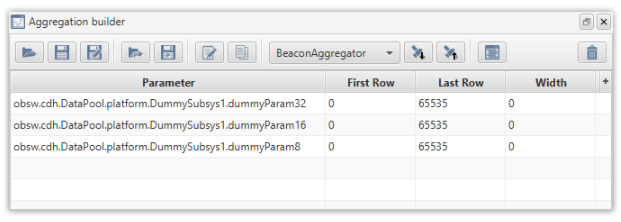
New aggregations are defined by dragging and dropping parameters from the mission explorer into the aggregator. You can add, modify, move, and delete parameters from aggregation definitions using this tool. If a parameter which has been added has a red background, it is ineligible for inclusion in that aggregation.
Existing definitions can either be loaded from files or downlinked directly from an onboard aggregator component if MCS is connected to the onboard software. Aggregation definitions can also be uploaded directly to an onboard aggregator component. An aggregation can be used by multiple aggregator components in the current asset deployment, and the drop-down list in the aggregation builder allows you to select from the available onboard aggregator components for uploading or downloading.
| You must associate an aggregation with an on-board component in order to uplink it. If you attempt to uplink it and have not selected an aggregation component, an error message will spawn saying "Could not find selected aggregator". |
Aggregations can be saved in a portable YAML format by clicking the save to portable format button. Saving your definition into the portable YAML format does not imply anything as far as the MCS is concerned; it will not use that aggregation definition until you register it with the MCS as a housekeeping aggregation.
Each selected parameter has four options, the first being Time field. This allows you to select from a drop-down of three options: no time, coarse time, and fine time. Selecting no time means that the aggregation will hold not record a timestamp for that parameter. Coarse and fine time will both hold a timestamp, with integer or long accuracy respectively. The second and third options, First Row and Last Row, are used to specify which rows of a multi-row parameter are aggregated. The Last Row cell will be automatically populated with the length of the parameter. Finally, the Width column is used to specify the bitwidth.
12.2. Associating aggregations with Beacons
Before the MCS will use a specific aggregation to decode incoming beacon packets or stored log files, you must first register your aggregation definition with the MCS as a named aggregation. You can do this either directly from the aggregation builder tool using the OK button, or from a YAML file using the New from file… context menu item on the aggregations node in the mission explorer.
Once you have registered your aggregation with the MCS, you can associate it with a beacon structure ID using the New mapping… context menu on the Beacon map node in the mission explorer, as shown in Figure 72. A window will appear which allows you to scroll between different beacons and select which aggregation to associate with each, as in Figure 73.
Beacons which already have an association are highlighted, and attempting to override the association will result in an error message. To re-associate a beacon, you must first delete the association through the Delete Mapping option in its context menu, then select a new one as above.
|
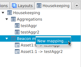
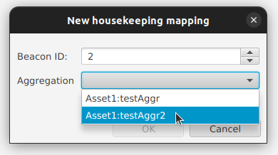
13. Decoding data
This section details the decoding of data received from the OBSW. Data is packed and stored in the channels of the Storage component, and must be downlinked and decoded in order to be human-readable.
13.1. Event Log Decoding
Going to Tools → Decode event log will bring up the window to decode an EventLogger’s contents, as displayed in Figure 74. The tool can decode either the data from a recent parameter get or downlink. Once decoded, the output can then be ingested into the MCS archive or exported as a Comma Separated Value (CSV) file to be loaded into a spreadsheet.
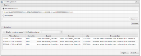
13.2. Data Log and Aggregation Decoding
Similar to event log decoding, it’s possible to decode the output from a DataLogger. As with the event log decoding, you can use either the values from a recent parameter get or from a downlinked binary file. The Data log decoder is accessed via Tools → Decode data log.
DataLoggers typically use the output from aggregators. Therefore, to decode a DataLogger, the corresponding aggregation is required. This can be supplied either by selecting an aggregation from the drop-down menu. Alternatively, an aggregation definition YAML file can be supplied (which can be generated using the aggregator tool).
Once you have set a source and definition, you can decode the source. The output should be similar to Figure 75.
By right-clicking selected data you will have the option to ingest, export or quick view the data in a map or a graph.
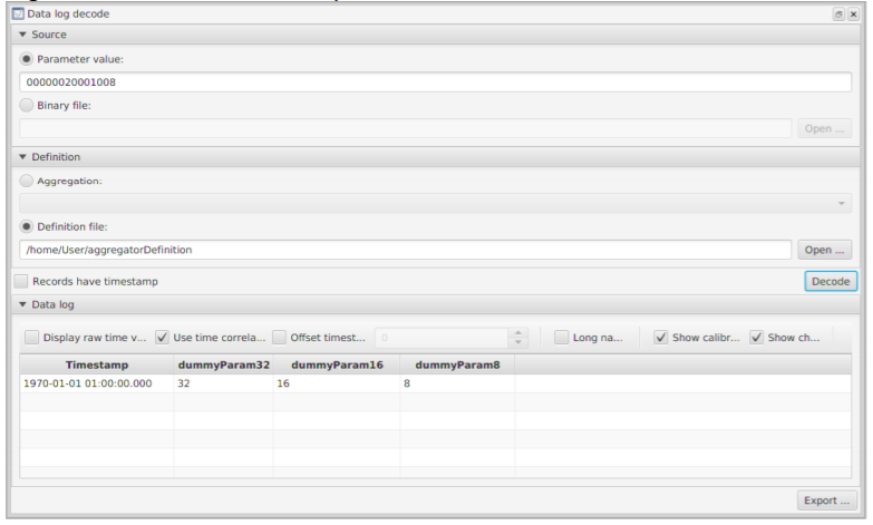
14. Archiving
This chapter details the archiving abilities of the MCS. Information is archived in two possible ways, firstly a main binary archive, and secondly as CSV files for specific cases. Archivers can be viewed and enabled in Housekeeping → Manage archive stores.
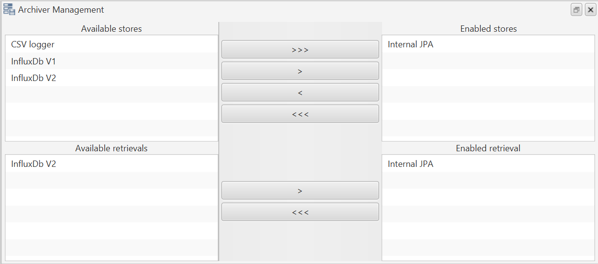
14.1. Main archive
The main MCS archive provides an historic store of all sent and received frames, packets, aggregations, parameters, check results, received events, actions requests, and their evolving execution status.
Options for the main archive currently extend to JPA or InfluxDB. JPA will be enabled by default for both storing and retrieving unless configured otherwise on start-up of the MCS. All possible archivers can be viewed and managed via the GUI as shown in the Figure 76. Multiple archives can be set as an enabled store by selecting the relevant arrows to enable them. However, only one or zero retrieval archives can be enabled at any given time. JPA doesn’t require any configuration parameters to be set, but the relevant parameters must be configured (Section 11.1.4) in order to use InfluxDB in the mcs.properties file. Currently there are two different versions of Influx that are supported, InfluxV1 will work with version 1 of InfluxDB and is only supported for storing values. InfluxV2 is compatible with version 2 of InfluxDB and supports both storing and retrieving values.
You can access parameter log history through the Parameter log view and graph view, where date ranges for data can be selected and retrieved from the archive in order to be viewed.
14.2. CSV aggregation logging
For received aggregations it is possible to request that their received value be logged to CSV files. These CSV files are located in:
MCS_HOME/hkLogs
14.3. Log view archiving
The log view at the bottom of the main screen is continually archived to CSV files found within:
MCS_HOME/data/archive/*.csv
Each CSV file corresponds to the tab name in the Log view.
Scrolling within the Log view will pull logs from the archive depending on whether there are any logs before or after that point.
14.4. Activity archiving
Activity archiving is available so that a full history of activities is stored and can be viewed through the MCS. Information on activity history is accessible through the Activity log view (Section 4.7) or the Activity Gantt chart view (Section 4.8).
15. Time Correlation
Unless a spacecraft is using an on-board clock that is already synchronised to UTC, time correlation is needed to convert between ground UTC time and the clock used on-board. Depending on the type of clock, and how it is updated in hardware, there is also a significant chance it will drift relative to ground UTC.
The time correlation functionality within the MCS allows it to compensate for on-board clock drift and time epoch so that it can convert between ground UTC and spacecraft timestamps when processing items such as data/event logs and on-board schedules.
There are two types of time correlation supported by the MCS:
-
Timestamp conversion - to convert between UTC ground time and an onboard timestamp (in both directions)
-
Reception time compensation - to calculate the actual timestamp, using latency, of a received packet where there is no onboard timestamp available
15.1. Time correlation concept
The time correlation algorithm uses three parameters to convert on-board time to ground UTC time and back. These are:
-
Scaling – A scaling multiplier applied to any conversion between flight and ground seconds. This compensates for on-board clock drift.
-
Offset – A value, in milliseconds, to add to any received onboard time to calculate a ground time. This compensates for on-board clocks that are based on elapsed mission time (or number of seconds since a known UTC time).
-
Latency – A value giving the latency, in milliseconds, between a packet being sent from onboard to being received on ground. Used to calculate packet generation time based on receptions time where no better actual on-board timestamp is available.
The MCS calculates the true ground time of an onboard timestamp (OBT) (in seconds) using the following formula:
Latency is only used when there is no actual on-board timestamp to convert and a ground reception timestamp is used instead.
15.2. Time correlation calculation
The scaling and offset values are calculated by using two different OBT/UTC pairs:
-
Base-OBT – A baseline OBT timestamp in on-board seconds
-
Base-TS – UTC timestamps in milliseconds Unix-time of the same instant as Base-OBT
-
Calc-OBT – A second OBT timestamp, taken after Calc-OBT, in on-board seconds that is used to calculate the offset and scale
-
Calc-TS – UTC timestamps in milliseconds Unix-time of the same instant as Calc-OBT
The formula for the scale value is:
The formula for the offset value is:
In both formulas the 1000 value is used to convert from the seconds unit of on-board timestamps to the millisecond units of the ground timestamp values.
15.3. Time correlation procedure
The two time pairs, Base and Calc, are required for the time correlation calculation to work. The Base values should be set as soon as possible in the life of the mission, and the Calc pair updated periodically thereafter.
During the first contact an initial Base and Calc set of values should be obtained.
As the base and calculated values will have been obtained in a very short time period, external factors such as round trip time and communication jitter can have a disproportional effect. If the calculated scale value is not 1.0 the Calc values should be manually set using the following formulas:
-
Calc_TS=Base_TS+ 1000 -
Calc_OBT=Base_OBT+ 1
This will update the proposed scale to exactly 1.0.
The Base values should not need to be updated after this.
To correctly compensate for clock drift, i.e. update the scale part of the formula, the Calc values should be updated periodically (for example every few days).
It is best to perform the first iteration of this operation at least a few days after the setting of the Base values to allow the drift of the on-board clock to be significant enough to be detectable.
The scale should always be very close to 1.0, any other value would indicate an issue with the values received.
|
15.4. Configuring time correlation using the GUI
The time correlation GUI allows an operator to:
-
obtain new timestamp pairs from the OBSW
-
calculate a proposed scale/offset pair
-
and update the currently active scale/offset pair used by the MCS.
The GUI is opened from Tools → Show time correlation, and can be seen in Figure 77.
Among the displayed fields are the current values in the top Current settings pane, the proposed values in the bottom Proposed settings pane, and controls in the middle for obtaining updated values from the remote OBSW. The proposed values are pre-populated from the current settings.
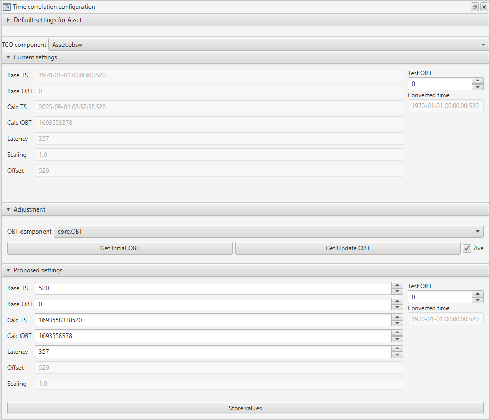
There is also a section at the top for 'Default settings', where we can configure time correlation settings at the asset-level by specifying a particular targets time correlation configuration to be used when a target is not supplied for an operation. When a target is supplied for an operation involving time correlation, that target will be used. The default value is only used when the system doesn’t have an alternative. Expanding this dropdown, we can see the target whose time correlation configuration is being used for the current asset. There is also an option below to select a different target in the dropdown to set that target’s time correlation configuration as the default being used for the asset.

The proposed Base TS and Base OBT values can be updated by using the Get Initial OBT button. This sends a request for the current time to the OBSW so the MCS must be connected to the remote OBSW. Once this value is set for a mission it is unlikely that it will need to be updated again.
The calculated TS and OBT can be updated using Get Update OBT. This will also update the latency value. Any change to any of the four values will update the proposed scale and offset parameters. This proposed value can be tested using the Test OBT option, which when populated will change the converted time in the box below to correspond to the given OBT.
To use the proposed values in the MCS the Store values button should be pressed, this will immediately apply the new settings for any future interactions with the remote OBSW.
|
15.5. Configuring time correlation using ground parameters
In situations where either the GUI approach is not available or not desired (i.e. to be managed via the Python API) the MCS offers a set of ground parameters for updating and maintaining the time correlation configuration. The parameters for the calculation are shown below:
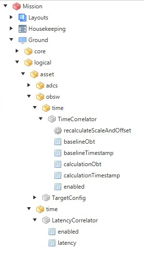
There is one set of time correlation parameters for each Target in the Asset, and a single latency value for each Asset. The full parameter name, for example as shown above, would be:
gnd.core:logical.asset.obsw.time.TimeCorrelator.calculationTimestamp
The recalculateScaleAndOffset action must be invoked for the new scale and offset values to be re-calculated from the updated parameters.
|
16. Ground Station Networks
MCS supports the use of third-party Ground Station Networks to connect to spacecraft. The configuration and credentials required to connect to any one of these networks depends on the specific third-party supplier. The following subsections describe how to set up MCS to use the networks which are supported as standard by MCS.
16.1. LeafSpace
To connect to satellites via the LeafSpace Ground Station Network, you must create a LeafSpace Connection Point via the MCS Mission Explorer. The context menu entry 'Add LeafSpace Ground Station Network…' on the Ground Station Networks tree item will display the LeafSpace Ground Station Network configuration dialog (Figure 80).
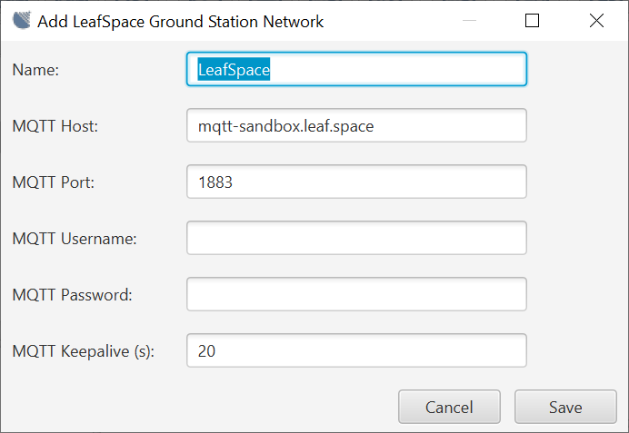
On Save, this will create a Connection Point which will be displayed under the Ground Station Networks node in the explorer, and which will provide a Connect option, to connect to the current Asset via the configured network.
The name must consist of a letter followed by one or more letters, digits and/or underscore characters. Also, the name must be unique among all Connection Points for the Mission. The remaining credentials are required in order to establish the MQTT data connections used by LeafSpace to exchange data packets with MCS, and should be provided by LeafSpace as part of their Mission onboarding process.
In addition to the Connection Point configuration, any Asset which is to be connected via the LeafSpace network must be configured with a NORAD ID. This is done via the Asset properties configuration dialog (Figure 81). The NORAD ID is used by LeafSpace to derive the MQTT topic names (channels), through which data is passed to and from a given Asset.
The Uplink Frequency and Downlink Frequency settings, if non-zero, are used to communicate the required radio frequencies to LeafSpace when establishing a connection, where the frequencies normally associated with the configured NORAD ID (and shared with LeafSpace during onboarding) are not to be used for the Asset. LeafSpace enforces controls on the frequencies used for communications, to ensure that only licenced frequencies are used.
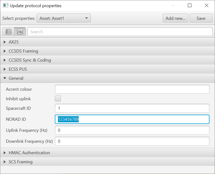
16.1.1. LeafSpace High-Speed UDP Connection Points
To set up a UDP server to received high-speed data from LeafSpace connections, select the 'Add Connection Point' context menu item on the LeafSpace Ground Station Network Connection Point. This displays the configuration GUI (Figure 82) allowing you to specify the UDP port and framing protocol(s) to be used with received data. This Connection Point type can also be configured to reconnect on failure.S
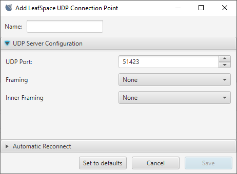
The first Framing selection should be set to match the framing employed by LeafSpace to send data to the UDP server. The optional inner framing selection should be set if the data extracted from the frames sent by LeafSpace is expected to be encapsulated in a framing protocol.
16.2. KSat
16.2.1. Connection Point Configuration
To connect to satellites via the KSat Ground Station Network, you must create a KSat Connection Point via the MCS Mission Explorer. The context menu entry Add KSat Ground Station Network… on the Ground Station Networks tree item will display the KSat Ground Station Network configuration dialog (Figure 83).
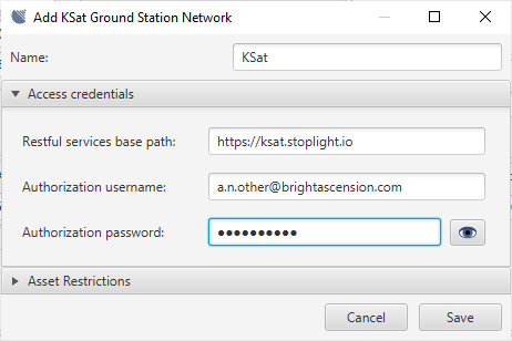
On Save, this will create a Connection Point which will be displayed under the Ground Station Networks node in the explorer, and which will provide a Connect option, to connect to the current Asset via the configured network.
The name must consist of a letter followed by one or more letters, digits and/or underscore characters. Also, the name must be unique among all Connection Points which appear directly under the Ground Station Networks and Direct nodes in the Connections explorer. The remaining credentials are required in order to access the KSat RESTful API which is queried during the Asset connect sequence, to provide real-time service availability information, and should be provided by KSat as part of their mission onboarding process.
The KSat connection process requires MCS to establish direct TCP/IP connections to KSat ground station antennae, over predefined IP addresses and TCP ports. You must create and configure individual KSat Direct Connection Points, parented on the KSat Ground Station Network Connection Point. Separate Connection Points must be created for uplink (TC) and downlink (TM) connections. Selecting the context menu item Add Connection Point on the KSat Ground Station Network connection point will raise the Add KSat Direct Connection Point dialog, in which the connection type of the new child connection point can be selected. After they are created, the child connection points are displayed in the mission explorer as descendants of the KSat Ground Station Network node (Figure 84).
For general TM and TC connections, a TCP Client Connection Point is required, and must be configured with an Antenna name as returned by KSat’s RESTful API during the connection sequence. A TC or TM framing option must be selected (see Figure 85), as agreed with KSat during the project on-boarding process.
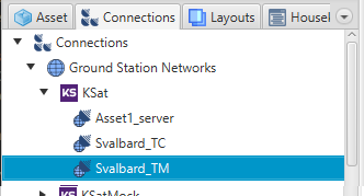
| An optional inner framing option should be set if the transmitted data will be in frames prior to framing for transmission. |
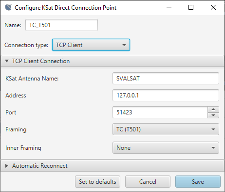
For high-speed (X-band) data download connections, a TCP Server Connection Point is required for each relevant Asset (see Figure 86). High-speed data received from a satellite will be streamed by KSat to a TCP server at an address and port agreed with KSat during mission onboarding. The port configured here must match that agreed port for the named satellite (Asset), and the satellite name given to KSat must match the Asset name. Also, the TCP server address agreed with KSat must match the MCS server’s public IP address. The framing for these connections is set to the predefined framing used by KSat for high-speed data transmissions. The optional inner framing options should be set if needed, as for TCP Client Connection Points.
| The names of the direct Connection Points are subject to the same character set limitations as other Connection Points. However, they are only required to be unique within the set of direct Connection Points with the same 'parent' Ground Station Network Connection Point. Therefore, it is valid for two KSat Ground Station Network Connection Points to have 'child' direct Connection Points with matching names. |
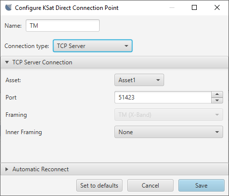
16.2.2. Opening Connections
Once the KSat Ground Station Network and Direct Connection Points have been configured, a connection to the current Asset can be opened via the Connect context menu item on the KSat GSN Connection Point or on its individual Direct Connection Points. Confirming the connection request triggers a request to the KSat RESTful Activity API, to supply a list of currently available services and antennae for communicating with the current Asset. On receipt of this information, MCS will open connections on the Direct Connection Points matching the available services. For example, if an Uplink service is available via a given antenna, and a TC Connection Point has been configured for the named antenna, MCS will initiate a connection via that Connection Point. TCP Server Connection Points are matched by Asset name rather than Antenna, and any configured for the current Asset will also be started, ready for data streamed from the KSat network.
| When testing a TCP Client KSat Direct Connection Point, you can leave the Antenna name blank, and the MCS will immediately attempt to connect to the configured TCP endpoint, bypassing the RESTful service. |
16.3. InfoStellar
To connect to satellites via the InfoStellar Ground Station Network, you must create an InfoStellar Connection Point via the MCS Mission Explorer. The context menu entry Add InfoStellar Ground Station Network… on the Ground Station Networks tree item will display the InfoStellar Ground Station Network configuration dialog (Figure 87).
On Save, this will create a Connection Point which will be displayed under the Ground Station Networks node in the explorer, and which will provide a Connect option, to connect to the current Asset via the configured network.
The name must consist of a letter followed by one or more letters, digits and/or underscore characters. Also, the name must be unique among all Connection Points for the Mission. The default host and port values reflect the standard location of InfoStellar’s StellarStation API server, and should typically be left unchanged. The Framing option depends on your mission-specific configuration.
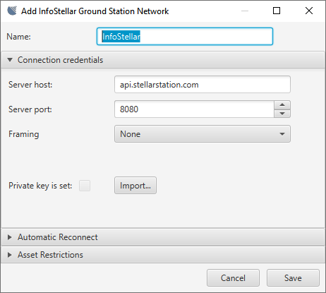
The StellarStation API requires credentials in the form of a private key. This must be imported from a key file which has been generated using the StellarStation web console.
In addition to the Connection Point configuration, any Asset which is to be connected via the InfoStellar network must be configured with a StellarStation Satellite ID. This must be stored as a custom property named StellarStation ID via the protocol properties configuration dialog (Figure 88). The required ID value is listed on the information page for the satellite in the StellarStation web console.
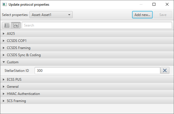
Use the Add new… button in the protocol properties dialog to create the custom property.
|
17. Export and Import
Selected configuration items can be exported to and imported from a file, as a means of backing up configuration settings, or of sharing them between MCS servers.
17.1. Export
To export configuration items, go to File → Export configuration in the MCS Display client. Figure 89 shows the export dialog which is displayed. All items can be included or excluded from the export by clicking on the relevant category checkbox. Items can also be selected or deselected individually. An optional description can be saved in the export file by filling in the field at the top of the dialog.
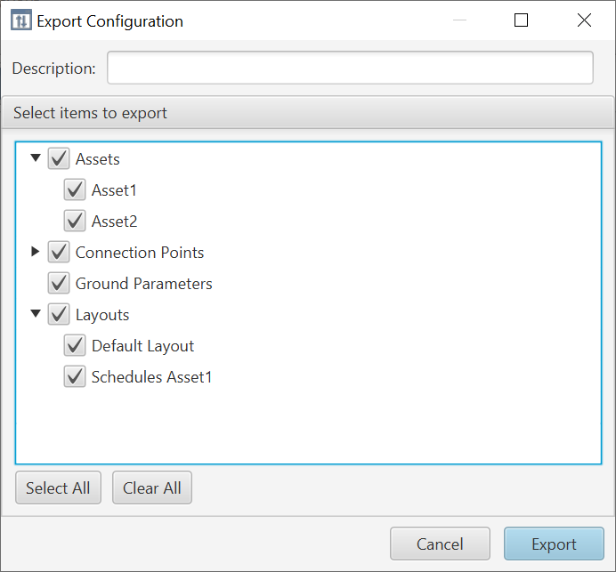
The exported asset information includes targets, asset and target protocol properties, deployments, aggregations and beacon maps, and logical Ground parameters for the selected asset(s).
Where connection points are organised into groups, only the group item is listed in the connection points selection list for each group. If a group is selected, the group item and all connection points in that group will be exported.
In the initial implementation, security association files for SDLS or space packet security protocols are not included in the export. However, any references to security association files are included, and these are retained on import if they are valid on the destination server. If they are not valid (for example, when setting up a new server), security association files need to be imported separately, via the Configure asset… option on the relevant assets.
When the export button is clicked, you are prompted to select a destination for the export file. A default filename is generated, which you can override as desired. On successful completion of the export, a confirmation is displayed, as shown in Figure 90.
17.2. Import
To import settings from a previously exported file, go to File → Import configuration in the MCS display client. A file selection dialog allows you to select a previously exported file. Figure 91 shows the import dialog which is displayed when a file has been selected. This displays the description which was input during export, along with the client system username of the user who created the export file, the export timestamp and the format version of the export file.
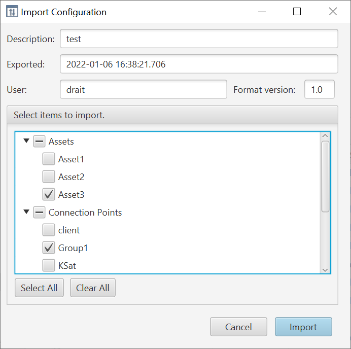
| The format version is in the form of a major.minor number pair. A system can import from any exported file with a major version number not greater than that generated by the system itself. Files with a higher minor version number may include data that the system will ignore. If an export file has a higher major version number than a system’s own exports, then the system cannot import items from that file, and a warning is displayed in the import dialog. |
You can select a subset of items to import from the file. Items which already exist in the server (matched by name) cannot be selected. If you try to select any such item, the checkbox remains deselected and a warning message is displayed in the selection pane title (see Figure 92).
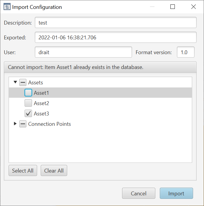
When you activate the import button, a progress bar is displayed as the selected items are imported to the server. As each item is imported, it is displayed in the mission explorer. On successful completion of the import, a confirmation is displayed, as shown in Figure 93.
18. Synthetic Parameters
By now, the concept of parameters and their role within the system should be familiar. So far, all the parameters encountered have been pre-defined in the SCDB. Their qualities, such as their name or associated component, can’t be changed in the MCS. Read-only parameters can’t be modified at all, while some parameters can have their values both read and set. By design, little control is exerted by the user over the parameters, primarily due to the well-defined nature of the SCDB.
Synthetic parameters differ from this in that they are not defined in the SCDB, but are fully defined in the MCS. They derive their values from one or more other parameters within the system, be those pre-defined in the SCDB, or synthetic. They are always read-only. In other words, they cannot change their source parameters, only read and manipulate them to produce useful outputs. This can support the definition of monitoring metrics, or key performance indicators, which are based on some transformation applied to one or more pre-existing parameters. A key difference between synthetic parameters and the calibrations encountered in an earlier chapter is that synthetic parameters can use any number of parameters in a more flexible way, whereas calibration involves set operations performed on one single parameter.
There are two steps to building a synthetic parameter: defining it and instantiating it. Specifying a synthetic parameter definition involves giving the MCS essential information about how to make a particular parameter. Instantiating then takes a definition and uses it to create a parameter occurrence in the mission tree, which can be accessed in the same way as any other read-only parameter. A definition can be used multiple times if necessary, for example for two different assets. The following sections will take you step-by-step through creating a definition and instantiating a synthetic parameter using that definition.
| Synthetic parameters are available to users of the MCS with a Professional, or Enterprise edition licence, which also has the Synthetic Parameter module. |
18.1. Synthetic Parameter Definitions
18.1.1. Definition format
Synthetic parameters can be defined in the MCS itself, through the synthetic definition manager under the Tools menu. They can then be saved to a YAML file and easily re-used in future sessions. Alternatively, synthetic parameters can also be defined directly in a YAML file and imported through the same manager. Each individual definition must have the following fields:
-
name: represents the parameter in the MCS
-
definition: describes the data type
-
expression: specifies how the value is generated
It is generally good practice to give synthetic parameters a descriptive name which allows them to be easily identified, including making it clear whether they are asset- or mission-level.
18.1.2. Synthetic Parameter Definitions
The MCS supports the definition of three different types of synthetic parameters: boolean, integer and floating point. The latter two must also have a bit-width specified, for memory efficiency. Examples of the different parameters are shown below.
definition:
type: booleandefinition:
type: integer
width: 8|16|32|64definition:
type: real
width: 32|6418.1.3. Synthetic Parameter Expressions
The expression section of a definition specifies how a synthetic parameter created from a given synthetic parameter definition will calculate its value. An expression is a string comprised of keywords and operators which can be evaluated and return a value. In the MCS, expressions are evaluated with respect to their expected type, so should be given a valid definition, and where source parameter values are available return a value of that type. Below is a short description of the available functionality within synthetic definition expressions.
Parameter Access
Parameter access is enabled via the parameter access service within the expression language of the MCS. Specifying svc.param('obsw.platform.DummySubsys1.dummyParam8') within an expression tells the MCS that when it evaluates the expression it should replace svc.param('obsw.platform.DummySubsys1.dummyParam8') with the most recent archived value of the parameter identified by obsw.platform.DummySubsys1.dummyParam8.
The MCS supports two kinds of synthetic parameter definitions: asset-level and mission-level. Asset synthetic parameter definitions may only reference parameters from a single Asset. Parameters referenced in Asset synthetic definitions should use the Asset and Deployment agnostic form of Element Identifiers such that they can potentially be instantiated on multiple different Assets. As an example, if the fully qualified identifier for a parameter called dummyParam8 on an Asset called Asset1 is Asset1.obsw.deployment:platform.DummySubsys1.dummyParam8, the Asset and Deployment agnostic form of that parameter identifier, which would be used in the synthetic parameter expression, is obsw.platform.DummySubsys1.dummyParam8.
Mission synthetic parameter definitions define synthetic parameters which are to be made available at the mission level. As such these definitions need to unambiguously reference parameters across all Assets included in a mission. Thus, they must use the fully qualified form of parameter names, e.g. Asset1.obsw.deployment:platform.DummySubsys1.dummyParam8.
| At present, it is not possible to use multi-row parameters to specify synthetic parameter expressions. Only single-row parameters are available for use. |
Arithmetic Operators
Standard arithmetic operations are supported, including addition (+), subtraction (-), multiplication (*), and division (/). As an example, to take the average of two parameter values, the following expression could be used:
"((svc.param('obsw.platform.DummySubsys1.dummyParam8') + svc.param('obsw.platform.DummySubsys1.dummyParam16')) / 2)"The above example also demonstrates that brackets can be used to group expression elements within a calculation.
Relational Operators
The following common relational operators are supported:
| Operator | Operation |
|---|---|
|
Equality |
|
Not equal |
|
Greater than |
|
Greater than or equal to |
|
Less than |
|
Less than or equal to |
As an example to test that one parameter has a value greater than an other the following expression could be used:
"svc.param('obsw.platform.DummySubsys1.dummyParam8') > svc.param('obsw.platform.DummySubsys1.dummyParam16')"Assuming its definition was created with a type of boolean, the above expression would evaluate to true if dummyParam8 has a value greater than that of dummyParam16, otherwise it would return false.
Logical Operators
The following logical operators are supported:
| Operator | Operation |
|---|---|
|
Logical and |
|
Logical or |
|
Not/boolean inversion |
As an example, to determine whether two boolean values are true, the following expression could be used:
"svc.param('obsw.cdh.logging.EventLogger.enabled') and svc.param('obsw.cdh.logging.BaseLogger.enabled')"Assuming its definition was created with a type of boolean, the above expression would evaluate to true if both EventLogger and BaseLogger are enabled, otherwise it would evaluate to false.
Mathematical Functions
The following mathematical functions are supported:
| Operator | Operation |
|---|---|
|
Raises |
|
Natural logarithm (logn) of |
|
Logarithm to base 10 of |
|
Raises Euler’s number to the power of |
Collection Functions
It is possible to specify a collection as part of an expression. The syntax for doing so is to surround a set of parameters in square brackets [] e.g. [svc.param('obsw.platform.DummySubsys1.dummyParam8'), svc.param('obsw.platform.DummySubsys1.dummyParam16'), svc.param('obsw.platform.DummySubsys1.dummyParam32')] or [1, 2, 3, 4]. The most recent cached version of each parameter in the collection is retrieved, and any any methods are applied to the resulting set.
The following collection functions are supported:
| Operator | Operation |
|---|---|
|
Returns the maximum value of the parameters in the collection |
|
Returns the minimum value of the parameters in the collection |
|
Returns the mean value of the parameters in the collection |
|
Returns the median value of the parameters in the collection |
|
Returns the standard deviation of the parameters in the collection |
As an example if the values of dummyParam8, dummyParam16, and dummyParam32 were, 8, 16, and 32 respectively, the following expression which calls max on a collection of those parameters, would return 32 as its value:
"max([svc.param('obsw.platform.DummySubsys1.dummyParam8'), svc.param('obsw.platform.DummySubsys1.dummyParam16'), svc.param('obsw.platform.DummySubsys1.dummyParam32')])"Conditional Operator
The conditional operator takes the form condition ? value_1 : value_2 and will return value_1 where condition evaluates to true and value_2 where condition evaluates to false.
As an example the following expression would return 1 if EventLogger is enabled:
"svc.param('obsw.cdh.logging.EventLogger.enabled') ? 1 : 0"18.1.4. Optional Fields
Additionally, a definition may contain the following optional fields:
-
documentation: used to display information about the synthetic parameter
-
version: an integer which tracks the history of the parameter
Any information input into the documentation field is displayed in the documentation pane in the bottom left of the MCS display, where the documentation of a standard parameter from the SCDB is typically displayed. This field supports markdown formatting which is converted to HTML in same way as the documentation from the SCDB for a standard parameter. The version field supports manual version management of synthetic parameter definitions.
If the version field is included its value should be an integer that is greater than the previous largest version number used for that synthetic parameter definition. The MCS supports the inclusion of multiple versions of a given synthetic parameter definition simultaneously, with synthetic parameter instances which are not using the newest definition flagged in the synthetic parameter management interface. If the version field is not included, the version number will be automatically incremented by the MCS when adding a synthetic parameter definition with the same name as a previous one. It is assumed that the added definition is the next version of the existing parameter. Functionally, versioning allows the capability to overload a name with multiple similar definitions, and use any one of them.
18.1.5. Examples
-
  name: "obsw.example_standard_deviation"
  definition:
    type: real
    width: 64
  expression: "standard_deviation([svc.param('obsw.platform.DummySubsys1.dummyParam8'), svc.param('obsw.platform.DummySubsys1.dummyParam16'), svc.param('obsw.platform.DummySubsys1.dummyParam32')])"
-
  name: "obsw.example_max_int"
  definition:
    type: integer
    width: 32
  expression: "max([svc.param('obsw.platform.DummySubsys1.dummyParam8'), svc.param('obsw.platform.DummySubsys1.dummyParam16'), svc.param('obsw.platform.DummySubsys1.dummyParam32')])"
-
  name: "obsw.example_logical_and"
  definition:
    type: boolean
expression: "svc.param('obsw.cdh.logging.EventLogger.enabled') and svc.param('obsw.cdh.logging.BaseLogger.enabled')"-
name: "obsw.example_documentation"
definition:
type: real
width: 64
expression: "((svc.param('obsw.platform.DummySubsys1.dummyParam8') + svc.param('obsw.platform.DummySubsys1.dummyParam16')) / 2)"
# Example of including optional documentation field
documentation: |
# This will appear as a H1 headin
Multi-line string so allows for comprehensive documentation
version: 118.2. Managing Synthetic Parameter Definitions
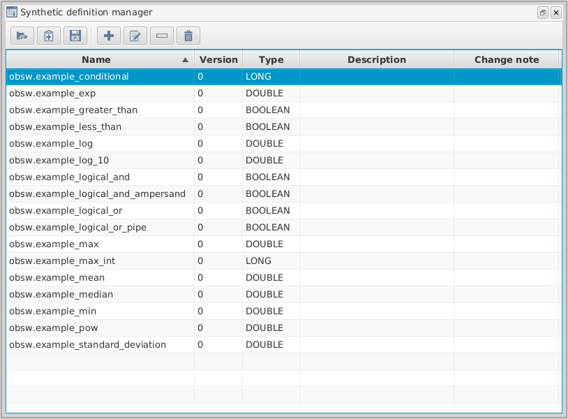
Synthetic parameter definitions can be managed via the synthetic definition manager tool, accessible from the Tools menu. This tool provides an overview of all synthetic definitions which have been imported in the MCS. Additionally, it provides functionality to:
-
import a new definition
-
import a new version of an existing definition
-
export a definition
-
add a new definition
-
modify an existing definition
-
rename an existing definition
-
remove a definition
Modifying a definition automatically increments its version number, but leaves the previous definition available with its pre-existing version number. This allows the introduction of multiple versions of the same definition, all of which can be used to create synthetic parameters.
Renaming a definition also increments its version number, and adds a change note indicating what the definition’s previous name was. It also flags synthetic parameter instances which are associated with the removed definition in the synthetic parameter management tool for potential deletion.
When a definition is removed, all versions of that definition are removed, and it is no longer available for creating synthetic parameter instances. Any existing instances which are associated with the removed definition are flagged with a red background in the synthetic parameter management tool for potential deletion. However, the MCS does not immediately "forget" the definition - if a new definition is loaded into the current session with the same name as one that has been removed, the new definition will automatically increment the version number from the removed one, instead of starting again from zero. This is to avoid confusion between previously removed and current definitions.

The synthetic definition editor can be accessed via the toolbar in the Synthetic definition management tool. The synthetic definition add dialog allows you to create new synthetic parameter definitions, without having to write and import a YAML file. The same rules apply as for definitions specified in a YAML file: a name, type and expression must be specified. Additionally, the expression must be validated before the definition can be added to the MCS.
The synthetic definition modify dialog is the same as the add dialog, except that it pre-fills the fields with information from the definition being edited. Any changes must also be validated before being permanently applied.

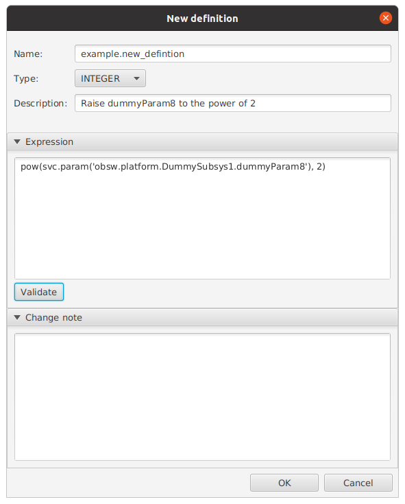
18.3. Synthetic Parameter Instances
Synthetic parameter definitions must be instanced in order to be accessible in the same way as other parameters. This is done through the synthetic parameter manager tool in the Tools menu. It provides a view of all the synthetic parameter instances for a given Asset or Mission, as well as functionality to:
-
Add new instances
-
Change the definition version
-
Update all instances which use a specific definition version to the newest version
-
Rename instances
-
Copy from one Asset to another
-
Delete instances
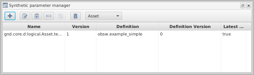
The drop-down menu at the top allows you to choose between viewing or associating a new synthetic parameter instance with the Mission or with an individual Asset. Once a choice has been made, clicking the add button brings up the add window, where new parameter instances can be defined.
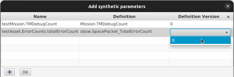
Each instance requires three fields: a name, a definition, and a definition version. The name must take one of two forms: subsystem.component.paramName or component.paramName. Note that synthetic parameter instances can be found under the logical subsection of the ground tree of the Mission Explorer, under either the relevant asset or mission subsection. Therefore, the subsystem and component names are not those of existing subsystems and components in the mission, but can be anything, and are defined by the user in order to better organise the parameters. Clicking on the definition cell of the parameter you’re instantiating will reveal a drop-down list of all valid definitions, from which one can be chosen for that instance. Finally, clicking the empty cell under definition version allows you to choose which is required from a drop-down of the versions of that definition.
| If you see an error that mentions an invalid name, make sure your name follows the conventions above. It must have at least one full stop. |
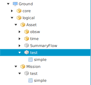
In the above figure two synthetic parameters have been created. One is an Asset synthetic parameter called "simple" and can be found in the ground logical tree under Asset > test > simple. The other is a Mission synthetic parameter, also called "simple", and can be found under the ground logical tree under Mission > test > simple.

You can interact with synthetic parameters as you would any normal parameter, bearing in mind that they are always read-only. Getting a synthetic parameter will return its current value (if it has one). A synthetic parameter will only have a value if all of its source parameters have a value in the MCS archive. It will publish updates of its value if all of the source parameters have values, and an updated value is received for one of those source parameters.
Synthetic parameters have a fully qualified identifier which namespaces them under the ground logical tree, as well as the Asset, or Mission the parameter was created for. Adding a synthetic parameter with a name of test.simple to an Asset called Asset, will result in a synthetic parameter with a fully qualified identifier of gnd.core.d:logical.Asset.test.simple. By using their name in the same way as natural parameters, synthetic parameters can themselves be used to create other synthetic parameters.
19. Procedure execution
Procedure execution is a way of automating a set of service requests to be performed within the MCS (for example, invoking actions, setting parameters) with various constraints. It is a user-friendly way of automating nominal passes or general operations that requires no knowledge of programming. Outside of scripts being executed in procedures, procedures are entirely deterministic - there is no conditional logic in procedure execution, which makes it very easy to calculate the cost of a procedure in terms of time, power or data budgets, and plan a pass accordingly. It supports complex stacks and high-level tasks, and it is also possible to set up parent activities which indicate the relationship between actions.
Procedure execution is available to users of the MCS with a Professional, or Enterprise edition licence, which also has the Procedure Execution module.
19.1. Procedure definitions
A procedure definition defines what a procedure does. A procedure definition contains the set of service requests to be executed, specified at relative times, with other rules and constraints. The service requests available to automate within a procedure are finite, available services are listed in Section 19.1.3.
19.1.1. Defining a procedure
A procedure can be defined using a live editor in the GUI, or by directly creating one in XML format.
Procedure definitions are multi-target, so one procedure can communicate with multiple targets of the same asset. All entities, where an entity refers to the name of something for example parameter or an action, referenced in a procedure should be defined relatively, with no asset or target information. A target can be specified in a separate, optional field. The asset information for an entity is provided from the procedure instance ID upon execution, and the target will also be taken from this ID if it is not already specified in the service request.
A procedure definition is defined by the following information:
| Attribute | Details |
|---|---|
Name |
The name of the procedure definition, must be unique across all procedure definitions. |
Version |
The version of the procedure definition. A procedure definition of the same name can have multiple versions. |
Execution model |
How the procedure definition should be executed. Possible values are 'EXECUTE_ALL', 'STOP_ON_FAIL' and 'STOP_ON_TIMEOUT'. |
State propagation |
The state to propagate as the final state of the procedure after execution. Possible values are 'FIRST_FAILURE', 'LAST_FAILURE', 'FIRST_ENTRY', 'LAST_ENTRY', 'ALWAYS_COMPLETE', 'ALWAYS_FAILURE' and 'FALLBACK'. |
Description |
Optional - a description of the procedure definition. |
Arguments |
Optional - any arguments to be defined for the entire procedure and can be used in any number of entries. |
Entries |
At least one entry must be specified per procedure definition. See below for more information. |
Fallback |
Optional - one fallback option can be provided per procedure definition. If 'FALLBACK' is selected as the state propagation, then in the event that the procedure fails, the fallback will be executed, and the procedure definition will take the state of the fallback. A fallback is a single service request. |
19.1.2. Procedure definition entries
A procedure definition entry can either be a service request entry or a verification entry. A service request entry will contain a single service request to be executed, and a verification entry will contain one or multiple verifications which can either check parameter values or event occurrences.
| Attribute | Details |
|---|---|
Propagate fail |
Whether to propagate any failures in this entry up to the procedure definition. If set to false then the state of this entry will not matter to the procedure and if a failure happens in this entry then this will not feed into the state of the overall procedure. |
Start with previous |
Whether to start this entry with the previous entry. |
Time lag |
The time lag, in seconds, after which to start the entry. It can be started relatively from the entry before it, or from when the procedure is executed, depending on the 'start with previous' flag. |
Retry |
Optional - a procedure definition can be retried if 'maxRetries' (the maximum number of times to retry the entry) and 'waitPeriodSeconds' (the number of seconds to wait in between retries) are specified. An optional 'retryOn' field can be specified to only retry on timeouts or only retry on failures, if this is not set then the retry functionality will kick in on either a failure or a timeout. |
Service request entries
A service request entry will contain one service request to execute, with conditions. As well as the above procedure definition entry information, a service request entry has the following additional information:
| Attribute | Details |
|---|---|
Service |
Which service to use |
Operation |
Which operation in the service to use. |
Entity |
Optional - can be defined depending on the service request (for example, a parameter set will require the name of the parameter here) |
Arguments |
Optional - any number of arguments can be provided here as arguments to be passed to the defined service request. The arguments can be given values directly, or can take the value of an argument defined for the procedure definition. |
Assign |
Optional - the results of a parameter 'get' service request can be passed to a pre-defined argument in the procedure definition whose name matches that given by 'assign', this argument can then be used later on in the procedure with its new value as the result of the parameter get. |
Verification entries
A verification entry will contain one or more verifications, with conditions.
A verification can either verify that a parameter is a certain value by doing a parameter get, it can verify that the values of a group of parameters within a certain time frame by checking the value in the archive or checking any live updates, or it can check that an event has happened.
As well as the above procedure definition entry information, a verification entry has the following additional information:
| Attribute | Details |
|---|---|
Wait |
The time in seconds to wait to decide the outcome for each verification. |
Verifications |
A list of one or multiple verifications. A verification will contain a 'type' (either parameter or event), an ID (relative name of the parameter or event) and an optional value. A value is only applicable for parameter verifications, to check that a parameter has a certain value. |
Example XML
An example XML is shown in Figure 102. For more examples of what the XML should look like, procedures can be created in the live editor and exported into XML format for reference.
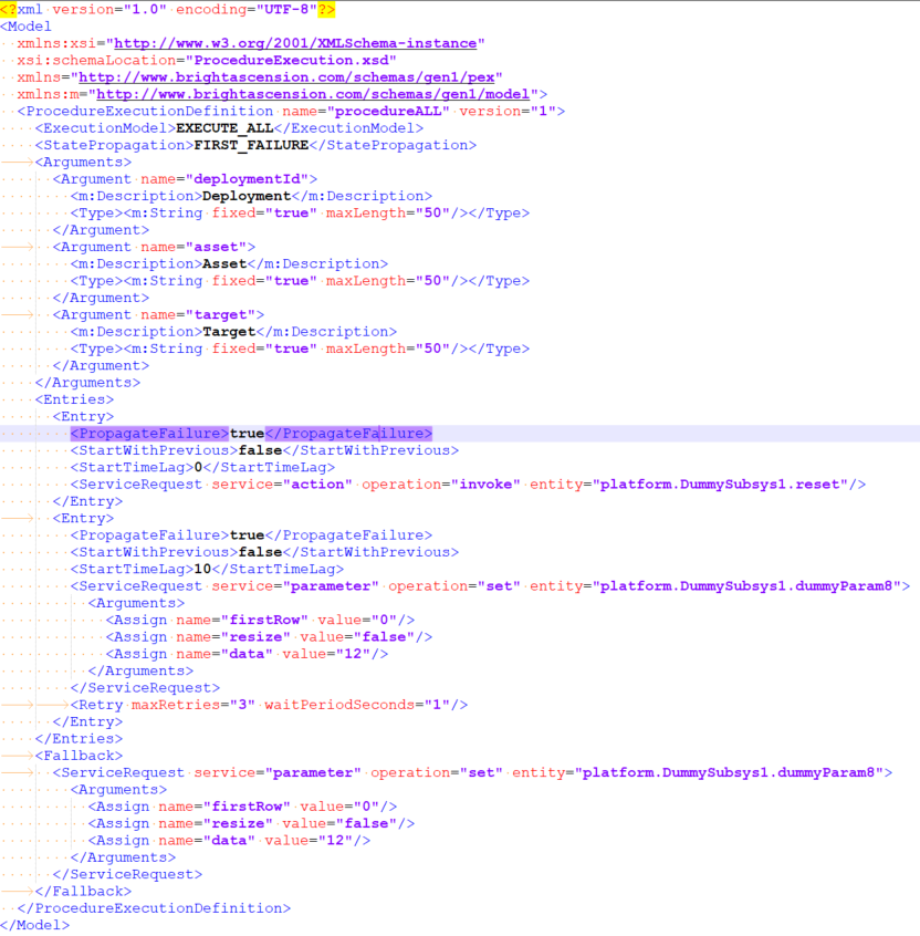
19.1.3. Supported service operations
The following section details which services, and operations within those services, are supported from procedure execution.
Procedure execution service
| Operation | Description | Mandatory arguments |
|---|---|---|
Execute |
Existing procedure instances can be executed inside of a procedure definition |
The procedure instance name should be provided in the 'entity' field and any arguments required by the procedure. |
Action service
| Operation | Description | Mandatory arguments |
|---|---|---|
Invoke |
Actions can be invoked inside of a procedure definition |
The action name should be provided in the 'entity' field |
Parameter service
| Operation | Description | Mandatory arguments |
|---|---|---|
Get |
Parameter values can be obtained inside of a procedure definition and the result of the 'get' can be stored in a pre-defined argument (within the procedure) using the 'assign' tag. |
The parameter name should be provided in the 'entity' field. Also required: 'firstRow' as an integer, 'lastRow' as an integer and 'resize' as a boolean. |
Set |
Parameter values can be set inside of a procedure definition. |
The parameter name should be provided in the 'entity' field. Also required: 'firstRow' as an integer, 'resize' as a boolean, and 'data'. |
Scripting service
| Operation | Description | Mandatory arguments |
|---|---|---|
Execute |
Groovy scripts can be executed inside of a procedure definition, which is where any operations not supported by procedures or any operations that require conditional or more complex logic should be executed from. |
'script' which should be the path to the script to be executed, and any other arguments required by the script. |
Activity service
| Operation | Description | Mandatory arguments |
|---|---|---|
Suspend |
Calling this operation inside of a procedure will suspend all transfers (including file transfers) |
None |
Resume |
Calling this operation inside of a procedure will resume all transfers (including file transfers) |
None |
Connection service
| Operation | Description | Mandatory arguments |
|---|---|---|
Add connection |
Connections can be defined inside of a procedure definition |
'connectionPointName' and 'connectionConfigURL' |
Open connection |
Connections can be opened inside of a procedure definition |
'connectionPointName', and 'useForSending' as a boolean |
Close connection |
Calling this operation will close all open connections to the MCS for the asset defined in the procedure instance |
None |
Transfer service
| Operation | Description | Mandatory arguments |
|---|---|---|
Uplink |
Parameter uplinks can be initiated inside of a procedure definition. This operation can take an optional argument, 'protocol', which specifies the preferred protocol to use for the uplink. If this is not specified then an appropriate protocol will be chosen |
The parameter name should be provided in the 'entity' field. Also required: 'firstRow' as an integer, 'lastRow' as an integer, 'resize' as a boolean, and 'filename' |
Downlink |
Parameter downlinks can be initiated inside of a procedure definition. This operation can take an optional argument, 'protocol', which is specified in the same manner as detailed above for 'uplink' |
The parameter name should be provided in the 'entity' field. Also required: 'firstRow' as an integer, 'lastRow' as an integer, 'resize' as a boolean, 'rowLength' as an integer, and 'filename' |
Multi-file downlink |
This works in the same way as the downlink above, but the downlinked content will be split across multiple files |
Requires above mandatory arguments for 'downlink' and 'rowsPerFile' as an integer |
File transfer service
| Operation | Description | Mandatory arguments |
|---|---|---|
Uplink |
File uplinks via CFDP can be initiated inside of a procedure definition |
The local source should be provided in the 'entity' field. Also required: 'localFilename', 'remoteFilename' and 'remoteDestinationString'. |
Downlink |
File downlinks via CFDP can be initiated inside of a procedure definition |
The remote source should be provided in the 'entity' field. Also required: 'remoteFilename' |
19.2. Procedure instances
A procedure instance is an instance of a procedure definition. A procedure instance consists of the name and version of the procedure definition to use and an ID. The ID should contain an asset identifier, a name and optionally a target identifier. The target is used to apply to any entries that don’t have a target specified. The name which can be defined in one of two ways - for example, 'procedure.uplink' and 'uplink' are both valid procedure names.
Multiple procedure instances can be created from a single procedure definition.
The concept of procedure instances and procedure definitions is similar to the synthetic parameters instance and definition concepts.
19.3. Procedure Management
Procedure definition and procedure instance management are available via the GUI and via the Python API.
19.3.1. Procedure Definition Management
The procedure definition management panel can be accessed in Tools → Procedure definition management, and looks like Figure 103.
In this display we are able to see an overview of all procedure definitions, we are able to add procedure definitions (either using the live editor or by uploading an XML file), as well as exporting, viewing, renaming, deleting and updating the version of a selected procedure definition.
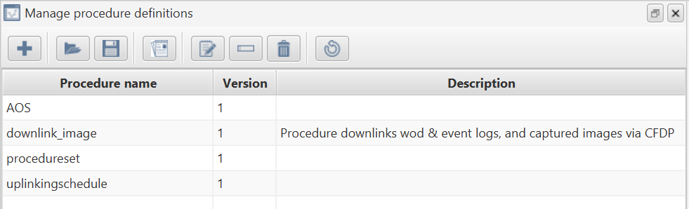
When a procedure definition is deleted, all versions of that procedure definition are deleted, as well as any procedure instances that use it.
Renaming a procedure will rename all versions of that procedure definition, and it will also update any procedure instances that currently use that procedure definition.
Updating the version of a procedure definition will allocate a new version number when an XML file is uploaded (new versions of existing procedure definitions can also be made using the live editor). The name in the uploaded XML file must match an existing procedure definition name.
19.3.2. Procedure definition editor
The procedure definition editor can be accessed via the toolbar in the procedure definition management panel, as shown in Figure 104.

This panel allows you to create new procedure definitions, and add new versions to existing procedure definitions, without having to go through the XML. Arguments can be copied and pasted from the top-level procedure definition to use as argument values for an entry, rows can be dragged and dropped on most tables.
To add entries, arguments or a fallback to a procedure definition, expand the relevant section below all of the basic procedure definition information. For entries, you must first specify whether your entry is a service request entry or a verification entry, and then double-click on the details column to add the detail of the entry. For service request entries, this looks like Figure 105.
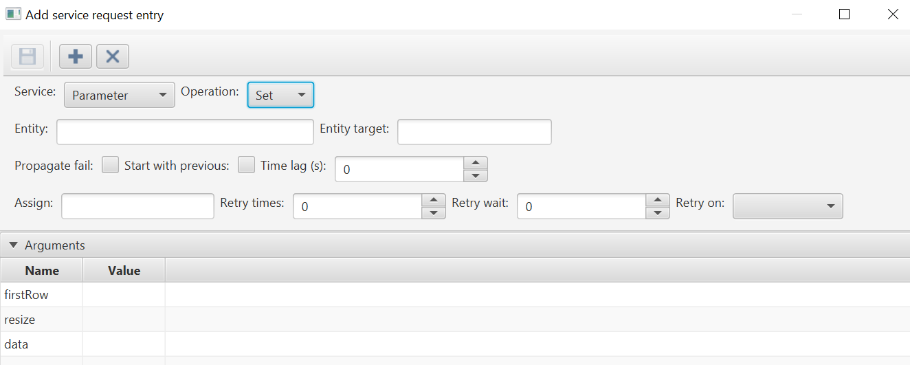
First, a service and operation must be selected, and depending on what is selected then a list of required arguments will populate in the arguments table below. These arguments must have values in order to save the service request entry. Arguments from the top-level procedure can be copied and pasted into rows in this table for use as argument values.
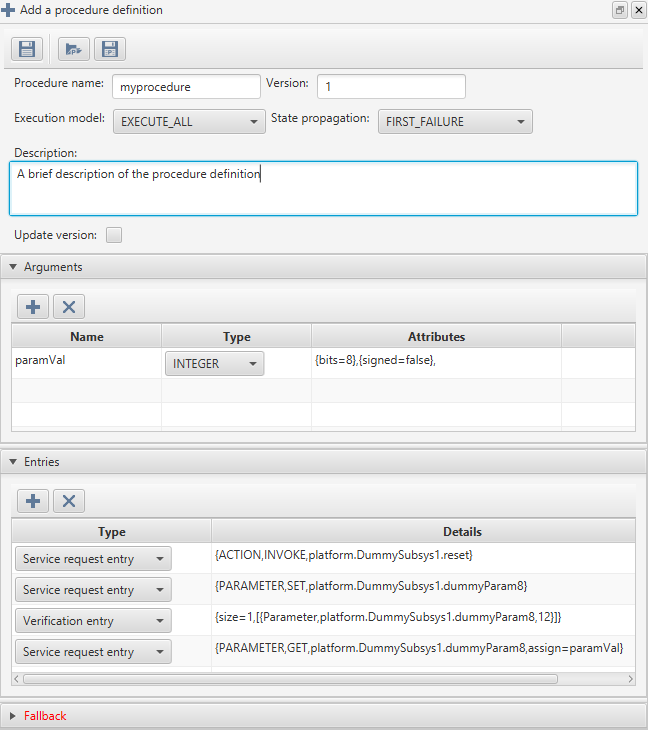
When a procedure definition is added, using the save button on the top left, a success message will pop up and the window will remain open.
To see the new procedure definition in the procedure definition management GUI, the refresh button can be used to update the table with any new procedures.
19.3.3. Procedure Instance Management
The procedure instance management panel can be accessed in Tools → Procedure management.
In this display we are able to see an overview of all procedure instances for a given asset using the asset dropdown, we are able to add new procedure instances, as well as updating the versions of procedure definitions being used by procedure instances, copying available procedure instances for one asset to another asset, renaming and deleting procedure instances.
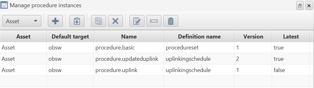
Procedure instances can be created from the + button, which will display a panel as in Figure 107.
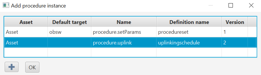
The Asset, Default target and Name fields are free text fields. The default target is the target to use for any entities in a procedure that do not already have a target assigned to them. For procedures interacting with a single target, the target can be set in this Default target field and it doesn’t need to be specified anywhere else. The procedure instance will be verified to ensure there are no entities that don’t have a target supplied, if one is not supplied in the default field then the procedure definition will be checked to ensure there are no entities without a target also specified. Then, a procedure definition name and version must then be selected from the dropdowns in order to create a procedure instance.
19.4. Executing procedures
Procedures can be executed from the GUI, by selecting the procedure instance from the mission explorer controller and double-clicking, or right-clicking and selecting Run. This will open up the procedure execution panel, as in Figure 109.

If the procedure requires any arguments, they can be provided in this panel before execution, as shown above. Documentation can also be viewed using the button on the far right, and clicking the arrow button next to it will execute the procedure.
Depending on if the procedure is successful, a tick or a cross will appear to the right in that panel.
Executing procedures can be viewed in the active tasks window and their status monitored, and any child activities as a result of a procedure can be seen in the same collapsible view as the top-level procedure.
Procedures can also be executed via another procedure, or via the Python API.